Uniaxial Bias Extension Test on Woven Engineering Fabrics

This protocol provides step-by-step instructions for conducting a reliable uniaxial bias extension (UBE) test. The UBE test is a commonly used technique for measuring the in-plane shear deformation of engineering fabrics and prepregs. The UBE test involves performing a tensile test on a rectangular specimen where the warp and weft directions are initially perpendicular to each other and orientated at ±45° to the applied tensile force (see Figure 1a). The specimen can be divided into three Regions A, B and C as shown in Figure 1. Region ‘A’ corresponds to in-plane pure shear, ‘B’ Regions undergo half of the shear of Region ‘A’ (if the yarns within the sample are inextensible and no inter-tow slip occurs during the test), and ‘C’ Regions remain undeformed. The aspect ratio, λ, the ratio between the width and height of the specimen, is considered to be at least two because it ensures that the pure shear is generated in Region A.

A displacement is applied across the UBE specimen, causing Region A to change from its initial square configuration (see Figure 1a - blue) to a rhombus (see Figure 1b – orange). The shear angle, θ, of the specimen can be determined by the dimensional change of Region A, as shown in the Figure 2.

θ is simply the difference between the initial inter-fibre angle (Φ₀) and the inter-fibre angle (Φ₁) at a given displacement, d.

                            θ = Φ<sub>0</sub>- Φ<sub>1</sub>                                                                                                              (1)

The ideal initial inter-fibre angle is 90˚. If the aspect ratio of the sample (λ) is greater than 2, Eq.(1) can be expanded [1], and the ideal shear angle can be calculated from Eq.(2) as,

                            θ = π/2 - 2 _acos_ [d/(2(λ-1) _LA_ <sub>A</sub>) +  _cos_ (Φ<sub>0</sub>/2)]                                                         (2)

Material

In this study, plain-woven glass fabric (see Figure 3a) with an areal density of 0.3 kgm^-2 was used to perform the UBE test. The weights of five samples (100 × 100mm²) were measured using a weigh-scale with 0.1g accuracy to calculate the average areal density. The average widths of the warp and weft tows were measured as 1.72 ± 0.09mm and 1. 76 ± 0.15mm (error represents +/- 1SD), respectively using the ImageJ software [2]. Also, the average gaps in the warp and weft directions were measured as 1.20 ± 0.11mm and 0.49 ± 0.13mm, respectively. These measurements were used in TexGen [3] to create Figure 3b.

Sample preparation

Prior to marking the sample outlines on the fabric, the fabric was placed on a flat surface (cutting board) and the fabric was manually adjusted to maintain the initial inter-fibre angle (angle between the warp and weft tows) at 90° (i.e., to avoid pre-shear). A parallel line to the weft tows was then drawn on the fabric, and a template was positioned at an angle of 45° to the drawn line (see Figure 4a). A specimen size of 400×200mm²was selected for this study. The template was adjusted to the required angle using a protractor. The outlines, gridlines, and diagonal lines in Region A (see Figure 1) were then marked using a black Sharpie pen (see Figure 4b). It is necessary to always mark the lines along a single tow for post-specimen analysis. The specimens were then cut along the marked outline using a rotary cutter (see Figure 4c & 4d). Use of a rotary cutter rather than scissors helps to minimize any pre-shear due to handling and produces a better finish along the edges of the samples. A horizontal line was marked across the back of the specimen (across the midsection) for the determination of the wrinkling onset angle.

The modified version of the UBE test involves bonding Aluminium (Al) foil to both the clamping region and 'Region C’ (see Figure 1) using epoxy resin. This allows easier drilling of holes and mitigates intra-ply slip during the test [4]. Therefore, another template was prepared based on the measurements

of the clamping area (30×240mm²) and Region C. The Al foil was folded in half and the template was positioned with the clamping area along the folded edge (see Figure 5a). The Al was then cut along the lines marked using the template. Using this method, both sides of the sections can be cut at the same time (Figure 5b).

The work surface should be prepared before applying epoxy resin (half of the cut Al sheet was inserted behind the sample - see Figure 6a) to protect other areas of the sample and the work surface from the adhesive. Using a nozzle glue gun, an appropriate amount of epoxy resin (Permabond ET500) was applied to the protruding half of the Al sheet (see Figure 6b). The resin was then evenly dispersed using a stick (see Figure 6c). In practice, pre-mixing the resin with disposable cups (see Figure 6d) is faster than using a glue gun with a nozzle because slow resin delivery from the nozzle can slow the process. It is important to thoroughly mix the resin and the hardener before applying to the specimen.

The adhesive was applied to both exposed sections of the foil at the same time (at either end of the specimen) and then attached to the sample. This technique involves applying the resin to the specimen in a semi-cured condition prior to bonding. The sample was then flipped, and the procedure was repeated. Make sure the adhesive covers only the 'C' regions and the clamping area, without contaminating regions A and B. Any glue on the rest of the sample will ruin the test specimen. The samples are left for 48 hours at room temperature to allow the epoxy resin to fully cure before drilling holes (to allow the sample to be mounted to the clamps). Figures 7a and 7b show the prepared UBE specimens prior to drilling and how the specimens should be stored for curing. Ten samples were prepared to perform the UBE test using two different setups (five repeats each) as explained in Section 2.4.

After 48 hours, holes were drilled, taking care not to deform the specimens (see Figure 8a). The completed specimen for the UBE test is shown in Figure 8b.

Loading and Clamping the Specimen

The UBE experiments were performed on a Zwick Z2 universal tensile testing machine mounted with a 2kN load cell (this test can be performed with any universal testing machine that has a load cell with sufficient resolution to accurately measure the relatively low forces involved in the test). The strain rate was set at 200 mm/min with a maximum upper force limit of 1000N. Force and crosshead displacement were measured by the test machine.

The UBE test was conducted using two different setups: with and without Anti-Wrinkle Plates (AWP). Five repeats of each test were conducted. Figure 9 shows the installation of the UBE test specimen in the test machine (without AWP). After installing the specimen, the initial inter-fibre angle should be verified prior to starting the test, to ensure that the pre-shear angle is less than 0.5°. This is a requirement for accurate results [5].

Setup using Anti-Wrinkle Plates: Two parallel Perspex plates with a 2mm gap were used for AWPs (see Figure 10a). The gap set between the Perspex sheets depends on the thickness of the fabric. In this study, the thickness of the specimen was below 2 mm even after bonding the Al foil. It is important to avoid contributions from friction, to the measured axial force. Prior to testing, the plates were cleaned using acetone. The AWPs were then placed in the middle of the two tensile testing clamps using three-finger double adjustment clamps fixed to two parallel stands mounted on the test bed (see Figure 10b). The plates were hinged on one side and the specimens were loaded by opening one plate of the setup. After installing the specimen the other side of the AWP was tightened using G-clamps (a low tightening pressure of 1Nm was used to maintain the 2mm gap between the two plates – see Figure 10c). Finally, the initial inter-fibre angle was again verified prior to starting the test (see Figure 10d).

Video setup

Manual image processing was used for post-test analysis. The front of the test specimen was filmed using a USB camera. The back of the test specimen was filmed using a smartphone camera positioned at an oblique angle (see Figure 11) to investigate the wrinkling behaviour of the specimens. The machine's force was set to zero prior to performing the test. The start button can be then pressed with the video capture option (synchronization of hardware allows for precise alignment between videos and test data, ensuring accurate frame-by-frame synchronization). If the machine does not offer the option of synchronous video capture, a manual method such as pressing the start button at the end of an audible countdown can be used. The countdown is audible so that the cameras can record it to allow the exact start point of the test to be found during post-test analysis.

Post-test, the videos were accurately cropped at the exact start of the test, using video editing software [6]. Locating the exact start point of the test is important as this is where the theoretical shear angle at a known displacement is determined in relation to the initial measurements of the specimen. The cropped videos (both front and back) were then converted to still frames using the software VirtualDub [7] and the frame rate was set to two frames per second (the frame rate of the videos is 30 frames per second, therefore every 15^th frame of the video is saved). VirtualDub is recommended for this analysis because it facilitates saving the exact required still frames, based on the frame rate of the video. The displacement between each still frame was calculated to be 1.6667mm because the strain rate was 200mm/min. In practice, it was found that there was a delay of two seconds for the sample to move after pressing the start button. This was evident from the fact that the first few still frames were identical. Therefore, the frame identified immediately prior to the first frame showing movement, was considered to be the initial frame of the test.

Image Analysis

The most important step in the post-experimental analysis of the UBE test is manual image analysis. ImageJ software [2] was used to measure the shear angle of each frame. The length of the clamp (240mm) was used to set the 'global scale' in ImageJ (see Figure 12), and the initial side length of Region A ( LA _A – see Figure 2) was measured.

When measuring inter-fibre angles, it is critical to minimise human error. Figure 13 shows the method used to determine the inter-fibre angle of the specimen. After loading the photo (still frame) to ImageJ, the picture was zoomed to the level of 400% where the image is shown as a set of individual pixels (see Figure 13a). The colour of the pixels in the middle of the drawn lines is darker than the pixels on the edges of the line. Thus, three points of the inter-fibre angle were traced across the middle pixels (dark colour) using the angle tool. When the cursor moves close to the traced point, the arrowhead of the cursor switches to a hand icon, as shown in Figure 13b. The exact coincidental line can be drawn by moving the traced point along the marked line on the specimen. Figures 13c and 13d show two measurements taken by adjusting only two endpoints of the drawn line (make sure that the two drawn lines are short and equal in length). This technique minimises the standard deviation of the measurements and enhances the reliability of the analysis. Figure 13e illustrates a perfectly drawn inter-fibre angle after zooming out. To improve the accuracy of the data, vertically opposing angles were measured (see Figure 13f) and the average was calculated. The inter-fibre angle was measured from each image as the test progressed until the crosslines in the middle of Region A became distorted, or difficult to measure due to wrinkle formation.

Wrinkle analysis

The obliquely angled back-camera video was split into still frames to investigate the onset of wrinkling. In this experiment, the wrinkle onset angle was determined by observing the horizontal line drawn on the back of the specimen (see Figure 14a). As the test proceeds, the horizontal line eventually becomes non-straight (see Figure 14b). The shear angle measured at that point is the wrinkle onset angle. The back camera was mounted at an oblique angle to observe the onset of the wrinkle. To obtain an accurate wrinkle onset angle, both front and back videos must be properly aligned with the start time of the test (time-synchronized).

Determination of the wrinkle onset angle is a challenge because the formation of wrinkles can occur in various ways (see Figure 15). Since the specimen is sensitive to small disturbances induced during the sample preparation, different wrinkle shapes can form at the same displacement, compare Figures 15a, 15b and 15c for examples. It is therefore important to define a robust method to identify the wrinkle onset angle. In this analysis, the still frames were moved backward from the end frame. At a given point, the non-linear centre line becomes straight. This point can also be observed in most cases (for glass fabrics) as Region A changes from a matte to a gloss appearance due to the disappearance of the wrinkle. Examples are provided in the supplied folder named "back". The frames '0032' and '00037' were selected as the wrinkle onset frames for setups without and with the AWP, respectively (see attached folders). The wrinkle onset angle was then determined using the corresponding front still frame (obtained from the time-synchronized front camera). To improve the accuracy of measurements, the inter-fibre angle was measured three times and the average value was used to estimate the wrinkle onset angle.

Measured versus theoretical shear angle

As shown in Figure 16, in-plane shear kinematics were measured for plain woven glass fabric with and without AWP. The inter-fibre angle was measured using the image analysis as described in Section 3.1 and the measured shear angle was then determined using Eq.(1). The theoretical shear angle at equivalent crosshead displacements were determined using Eq.(2). 'Ideal' shear kinematics, shown as the continuous black line in Figure 16, indicates pin-joined net kinematics where it is assumed that the fibres are inextensible and that there is no intra-ply slip [8]. The Excel file, attached in Section 6, provides calculations for two samples related to this analysis (i.e., without AWP and with AWP in sheet 1 and sheet 2, respectively).

The samples tested without the AWP produce a slight variation of data at the higher shear angles and the divergence of the measured shear angle continues until the angle becomes difficult to measure and therefore unreliable (see Figure 16a). In the AWP-free UBE test, the maximum measured shear angle is approximately 50°. However, the measured shear angles move towards the ideal line in UBE tests with AWP at higher shear angles (above 50°) and eventually fall below the theoretical shear angle (see Figure 16b) due to the growing influence of other modes of deformation, such as intra-ply slip [9]. The addition of AWPs reduces out-of-plane wrinkles and allows more precise measurements (less variance) of the measured shear angle, up to higher levels of shear (around 70°).

Normalised Force vs Measured Shear Angle

To increase the reliability of the measurements, the axial force is corrected by subtracting the force at the beginning of the test (i.e., before performing the test, it is necessary to adjust the force of the machine to zero. However, there may be a very small force acting on the specimen at the start of the test, often this force is minus. Therefore, when the samples are analysed, the initial force is more or less removed from the sample, see the attached spreadsheet). The force is normalised by dividing the initial side length of Region A ( LA _A), see sheets 1 and 2 of the attached Excel file. According to Figure 17, initially, the force required to deform the fabric is low and gradually increases with increasing measured shear angle, both with and without AWPs. At a moderate shear angle, around 30^o, the normalised force begins to increase rapidly. Due to the formation of wrinkles, the UBE test without AWP can only measure a shear angle of approximately 50° (see Figure 17a). At high shear angles (above 50°) the normalised force in the UBE with AWP increases very rapidly (see Figure 17b).

For better comparison between normalised force vs shear angle curves with and without AWP, the Y axis of the graph with AWP was replotted up to 60Nm^-1 (see Figure 18). The normalised force of the specimens with AWP shows a small increase at low shear angles relative to the specimen without AWP (see Figure 17a). For instance, the normalised force at the first displacement (1.6667 mm) of all samples without AWP was estimated to lie between 3-4Nm^-1 (see Figure 17a). However, the value is shown to be increased to 4-5Nm^-1 in the specimens with AWP except for specimen 2 (see Figure 18). The reason for this slight difference may be due to the frictional forces between the specimen and the AWP due to small misalignments.

Comparison of Test Results with and without Anti-Wrinkle Plates

Average curves of two experiments (with and without AWP) were plotted for comparison (see Sheet 3 of the attached Excel file for calculations). As shown in Figure 19a, the kinematics correspond closely until a measured shear angle of ~50°, after which AWP are required to collect further data.

Figure 19b shows the average normalised force versus measured shear angle curves with and without AWP. At shear angles above 40^o, the gradient of the average curve measured with AWP is greater than that of the average curve measured without AWP. This graph is scaled down to a maximum normalised force of 100 Nm^-1 for clearer comparison (see Figure 20). The reason behind the decrease in gradient for the measurements conducted without AWP is that the formation of wrinkles during the AWP-free UBE experiment, leads to apparent increases in the perceived shear angle, shifting the plotted data slightly to the right.

To overcome the frictional forces between the specimen and the AWP caused by misalignments (stated in Section 4.2) and to improve the reliability of the UBE test with more precise data, Harrison et al. [10] proposed combining shear angle data without AWP prior to wrinkle onset (below 30°) and shear angle data with AWP after wrinkle onset (above 30°). Blue dots in Figure 21 represent the plotted data points after combining with and without AWP data, in this analysis. The red line is the data-fitted 6^th-order polynomial trend line. Calculations combining with and without AWP data are provided in Sheet 4 of the attached Excel file.

Pre-shear Analysis

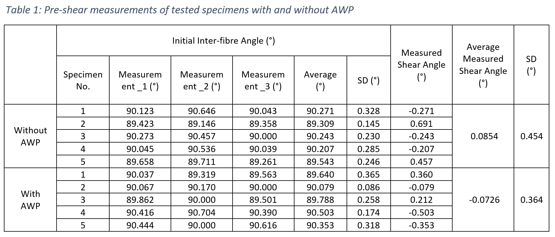
The initial inter-fibre angle of each specimen was always verified after the specimens were installed in the test machine. The first still frame was used during the image analysis to measure the initial inter-fibre angle and the pre-shear values are summarised in Table 1 for all the specimens tested. From each sample, three measurements were taken to determine the average value. According to the table, all initial inter-fibre angles are within a tolerance of 2°, and average pre-shear measurements are within a tolerance of 0.5° (except specimen 2 without AWP), as recommended by Alsayednoor et al. [5].

Wrinkle analysis

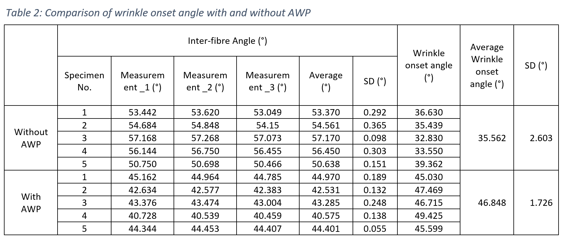
The measured wrinkle onset angles, both with and without AWP are shown in Table 2. According to the results, the wrinkle onset angle in the specimens with AWP occurs at a higher shear angle. The application of the Perspex screen can therefore delay wrinkle formation and increase the number of reliable data points that can be obtained. When comparing the wrinkle onset angle obtained in previous studies on the same fabric [10], the average wrinkle onset angle measured with AWP was found to be approximately the same (previously 46.4°, now 46.9^o); however, the standard deviation of the current results is significantly reduced when compared to the previous study (previously ~2.7˚, now ~1.7°). The reason for the difference may be the new inter-fibre angle measurement technique explained in Section 3.1.

Figures 22 and 23 show the specimens with and without AWP, both at 65mm of machine crosshead displacement. Due to the formation of wrinkles, the middle horizontal line on the back of all specimens tested without AWP is non-straight (see Figure 22). In contrast, specimens tested with AWP remain almost straight (see Figure 23).

Care should be taken to reduce the pre-shear of the fabric during sample preparation and loading of the specimen onto the test machine. Precautions for reducing pre-shear include careful handling of the fabric, initial manual adjustment prior to sample cutting and testing, and replacing regular scissors with rotary cutters for sample cutting. * When bonding the Al foil to the specimens with epoxy resin, great care should be taken to avoid contaminating the specimen outside of region C, which would ruin the viability of the specimen.

• It is best to perform at least four replicates of each test and average the results. To show the data distribution, error bars with +/-1 SD can be added to graphs.
• The captured videos should be accurately cropped. Finding the precise start point of the test is critical because all the calculations depend on the initial measurements of the specimen (i.e., initial inter-fibre angle, initial side length of Region A, and initial dimensions of the specimen).
• Several measurement errors can occur in the manual image analysis step. As mentioned in the literature, to obtain precise results, the standard deviation of the initial pre-shear angle should be less than 2°. According to the new approach explained in Section 3.1, the SD of measurements can be maintained within 1°. In addition, the inter-fibre angle can be measured three times to improve the accuracy of the UBE test measurements and the average can be calculated to obtain the shear angle at a given displacement.

To demonstrate the tests, videos and the corresponding still frames of the UBE test both with and without the AWP are provided. The reader is invited to download and analyse the videos and still frames, as described above. Your analysis can then be compared to the results that we created using these videos (provided in the attached Excel file).

UBE test without AWP for plain-woven fabric (Front) - PW_withoutAWP_Front.mp4

UBE Test without AWP for plain-woven fabric (Back) - PW_withoutAWP_Back.mp4

UBE test with AWP for plain-woven fabric (Front) - PW_withAWP_Front.mp4

UBE test with AWP for plain-woven fabric (Back) - PW_withAWP_Back.mp4

Still frames without AWP for plain-woven fabric (Front) - StillFrames_PW_withoutAWP_Front.zip

Still frames without AWP for plain-woven fabric (Back) - StillFrames_PW_withoutAWP_Back.zip

Still frames with AWP for plain-woven fabric (Front) - StillFrames_PW_withAWP_Front.zip

Still frames with AWP for plain-woven fabric (Back) - StillFrames_PW_withAWP_Back.zip

Excel file (calculations) - UBE_PW.xlsx

[1] P. Harrison, J. Wiggers and A. Long, “Normalisation of shear test data for rate-independent compressible fabrics,” Journal of Composite Materials, vol. 42, no. 22, pp. 2315-2344, 2008. https://doi.org/10.1063/1.2729646

[2] C. Rueden, C. Dietz, M. Horn, J. Schindelin, B. Northan, M. Berthold and K. Eliceiri, “ImageJ Ops [Software],” 2016. [Online]. Available: https://imagej.net/Ops.

[3] L. P. Brown, “TexGen,” in Advanced Weaving Technology. , Springer International Publishing, pp. 253-291, 2022. https://doi.org/10.1007/978-3-030-91515-5_6

[4] P. Harrison, “Modelling the forming mechanics of engineering fabrics using a mutually constrained pantographic beam and membrane mesh,” Composite: Part A, vol. 81, pp. 145-157, 2016. https://doi.org/10.1016/j.compositesa.2015.11.005

[5] F. Alsayednoor, F. Lennard, W. R. Yu and P. Harrison, “Influence of specimen pre-shear and wrinkling on the accuracy of uniaxial bias extension test results,” Composites Part A: Applied Science and Manufacturing, vol. 101, p. 81–97, 2017. https://doi.org/10.1016/j.compositesa.2017.06.006

[6] “support@123apps.com,” 16 May 2022. [Online]. Available: https://online-video-cutter.com/. [Accessed January 2023].

[7] A. Lee, “VitualDub 1.10.4.0. [software],” 2013. [Online]. Available: http://www.virtualdub.org.

[8] P. Harrison, F. Abdiwi, X. Z.Guo; P.Potluri; W.R.Yu, Z. Guo, P. Potluri and W. Yu, “Characterising the shear–tension coupling and wrinkling behaviour of woven engineering fabrics,” Composites Part A: Applied Science and Manufacturing, vol. 43, pp. 903-914, 2012. https://doi.org/10.1016/j.compositesa.2012.01.024

[9] P. Harrison, M. F. Alvarez and D. Anderson, “Towards comprehensive characterisation and modelling of the forming and wrinkling mechanics of engineering fabrics,” International Journal of Solids and Structures, vol. 154, pp. 2-18, 2018. https://doi.org/10.1016/j.ijsolstr.2016.11.008

[10] P. Harrison, E. Taylor and J. Alsayednoor, “Improving the accuracy of the uniaxial bias extension test on engineering fabrics using a simple wrinkle mitigation technique,” Composites Part A, vol. 108, p. 53–61, 2018. https://doi.org/10.1016/j.compositesa.2018.02.025