The role of artificial contact materials in experimental use-wear studies - "artificial vs. natural experiment"

Standardised tools

12 x 60°

12 x 60°

Raw material

Baltic flint:

Southern Sweden (secondary deposit):

55.945852 N, 12.767851 E

Silicified schist:

Balver Höhle (secondary deposit)

51.339167 N, 7.871944 E

Buhlen (secondary deposit)

51.191022 N, 9.086585 E

Blanks

Raw material nodules (step #1.1) were first cut into rectangular blanks of the following dimensions:

10mm

25mm

60mm

Equipment

Value	Label
Goliath 450	NAME
Lapidary rock saw	TYPE
Steinschleifmaschinen & Lapidary tools Ltd.	BRAND
-	SKU
-	SPECIFICATIONS

a) cut 10mm slices

b) cut slices into blanks

Hardness measurement

The hardness of the blanks (step #1.2) was measured with a Leeb rebound hardness tester.

Equipment

Value	Label
Equotip 550	NAME
Portable hardness tester	TYPE
Proceq	BRAND
-	SKU
Leeb C probe	SPECIFICATIONS

The blanks were placed on a stable base (here a flat rock slab of about 20kg). Since the samples did not fulfill the requirements for minimum sample size and weight, an additional coupling paste was used to connect the sample with the base. Each blank was measured ten times to insure and test intra-blank variability.

Edge angle

One end of the blanks (step #1.2) was cut to produce tools with a 60° , with the following dimensions:

10mm

25mm

30mm

Equipment

Value	Label
310 CP	NAME
Diamond band saw	TYPE
Exact	BRAND
-	SKU

Chamfered edge

To avoid catastrophic breakage of the edge during experiments, the leading edge of the samples (step #1.4) was chamfered at 45°.

Equipment

Value	Label
310 CP	NAME
Diamond band saw	TYPE
Exact	BRAND
-	SKU

The cut with the band saw left a small burr between the two adjacent surfaces at the edge of the chamfered surface and the lateral side D. This burr was manually removed with a mini diamond drill bit.

Not all 24 experimental standard samples were produced immediately. After the experiment was conducted with half of the samples, the length of the sample was reduced by removing a ~1 cm slice along the 60° leading edge to reveal a fresh, unused surface for a new cutting edge by repeating step 1.4 - 1.5. This way, 12 new samples could be produced without increasing raw material intra-variability.

Coordinate system

3 ceramic beads were adhered onto each side of the cutting edge to produce a coordinate system on either side.

For details, see:

Cleaning

100mL

1Mass / % volume

Equipment

Value	Label
Sonorex Digitec DT255H	NAME
Heated ultrasonic bath	TYPE
Bandelin	BRAND
-	SKU
4.5 L	SPECIFICATIONS

45°C

0h 10m 0s

Hard and soft contact material

Four different contact material were used: two natural and two artificial contact materials.

Natural contact material

Cow scapula ( Bos primigenius) was provided by a butcher in a fresh state. The periosteum and small pieces of flesh were still attached to the bone. The cutting experiment was carried out in a laboratory under ambient room temperature conditions. During the course of the experiment, the bone started to dry out but apart from desiccation no other degradation processes were visible. The bone was used as hard contact material.

Fresh pig skin ( Sus scrofa domesticus ) provided by a butcher by separating the skin from the flesh below. Experiments on the skin were conducted at room temperature. Overnight storage was executed in a refrigerator. Two pieces of skin were needed during the course of the experiment. The skin was used as soft contact material.

Artificial contact material

Synthetic bone plate with a rubber skin layer (imitating periosteum) with the following dimensions:

250mm

250mm

6mm

Shore hardness (D): 78 ± 5 %

Artificial skin made of silicone ecoflex. The skin pad has the following dimensions:

140mm

130mm

4.2mm

Shore hardness (A): 0-3

General settings

Linear unidirectional cutting movements: 2000strokes split in 4cycles .

The cycles are defined by the follwing number of strokes:

1strokes to 50strokes

51strokes to 250strokes

251strokes to 1000strokes

1001strokes to 2000strokes

Note: the stroke movement length on the soft contact material (and for some samples on the fresh cow scapula) was half the length compared to the stroke movement length on the hard contact material. In thoses cases, the number of strokes was doubled.

Experimental setup

Equipment

Value	Label
SMARTTESTER	NAME
Modular material tester	TYPE
Inotec AP	BRAND
-	SKU
recorded values with the time stamps:

• for each drive: position, speed, acceleration, force (as measured through the drive's current usage)
• penetration depth with extra sensor
• apllied force with extra sensor
• friction with extra sensor | SPECIFICATIONS |

Linear movement from start point to end point:

2kg / 6kg

100mm / 200mm

600mm/s

4000mm/s2

10Hz (for each data channel)

Setup sample holder

The length of the spring on the sample holder was adjusted to compensate for the weight of the sample holder itself (without dead weights and sample).

Adjust the position of the spring attachment on the rail, so that:

1. the sample holder almost touches the frame, and
2. at the same time, there should be no pull from the spring against the sample holder frame.

Setup sample

The sample (step #1) was clamped in the sample holder (SMARTTESTER) and manually orientated (i.e. angles corrected and standardised) in all directions.

The cutting edge was parallel to the plane of the contact material (90° )

Setup contact material

The contact materials were fixed onto the table in different ways. Each method guaranteed that the contact material could not move during the experiment. Additionally, after removing the contact material for scanning or overnight storage, repeated identical positioning was possible. The materials were aligned with the X-axis.

a) cow scapula

The cow scapula was aligned horizontally and fixed with three bolts on a wooden base (see images in steps #2.1 and #4.2). The wood itself was fixed with screw clamps to the table.

b) pig skin

The pig skin was fixed with two perforated metal strips on a wooden base (see image in step #2.1), which was fixed with screw clamps to the table.

c) bone plate

The bone plate (step #2) was clamped around the edges in a custom-made sample holder and fixed with a screw in the middle of the bone plate.

d) soft tissue pad

The soft tissue pad was attached with a double-sided adhesive tape to a plastic cutting board. The board itself was fixed with screw clamps to the table.

Program cutting movement

For each sample, a new template was created (named with the sample ID and the stroke number).

a) Move down in Z-direction to start position

The z-value of the starting point was defined as follows: the z-drive was moved down slowly until the edge of the tool was in contact with the contact material. A few extra mm (e.g. 5 mm for the bone plate) were added to the position of the z-drive in order to give the tool the possibility to penetrate into the contact material without cutting through it.

b) Move forward in X-direction 100mm / 200mm (linear movement)

c) Move up in Z-direction approx. 20mm (above bone plate; no contact between contact material and tool)

d) Move backward in X-direction to starting point

e) Loop 50 times over steps #4.1a-4.1d and export data to CSV

f) Loop 200 times over steps #4.1a-4.1d and export data to CSV

g) Loop 750 times over steps #4.1a-4.1d and export data to CSV

h) Loop 1000 times over steps #4.1a-4.1d and export data to CSV

The experiment was planned as a sequential experiment. The 2000 strokes were therefore split into four sequences (steps #4.1e-h). The tools were documented after each sequence (step #5).

For each sequence, five CSV files were exported, one for each recorded data channel:

• Sample penetration depth into contact material as measured by the distance sensor in the sample holder.
• Force applied (Z-direction) as measured by the force sensor in the sample holder with affixed dead weights.
• Friction as measured by the force sensor in x-direction between the stage and the fixed stage frame (between mounted contact material and sample).
• Position of the X-drive (travel range).
• Velocity of the X-drive.

cutting_template.Smart

Run program

• Each sample was used over a duration of ~ 7h 0m 0s (= running time SMARTTESTER)

The following samples were used for the experiment:

a) cow scapula

 FLT4-6

 FLT4-14

 FLT4-15

 LYDIT4-5

 LYDIT4-7

 LYDIT4-12

b) pig skin

 FLT4-4

 FLT4-12

 FLT4-13

 LYDIT4-1

 LYDIT4-4

 LYDIT4-6

c) bone plate

 FLT4-10

 FLT4-7

 FLT4-5

 LYDIT4-2

 LYDIT4-3

 LYDIT4-8

d) soft tissue pad

 FLT4-11

 FLT4-12

 FLT4-13

 LYDIT4-9

 LYDIT4-10

 LYDIT4-11

Sample documentation

Before the experiment, as well as after each cycle, all 24 samples were documented in an identical way following these steps:

• cleaning with tap water and comercial washing up liquid
• weight measurement (threefold repetition)

Equipment

Value	Label
Kern PCB 3500.2	NAME
weighing scale	TYPE
Kern	BRAND
-	SKU
accuracy of 0.1g	SPECIFICATIONS

• 3D scanning (identical settings for all scans)

Equipment

Value	Label
smartScan-HE R8	NAME
3D structured light scanner	TYPE
AICON	BRAND
-	SKU
S-150 FOV, resolution of 33 µm	SPECIFICATIONS

• cleaning with tap water and comercial washing up liquid
• optical documentation of three of the four surfaces per sample (one lateral and the two main surfaces)

Equipment

Value	Label
Smartzoom 5	NAME
digital microscope	TYPE
ZEISS	BRAND
-	SKU
1.6x objective; EDF-stitching images	SPECIFICATIONS

• cleaning the area of interest with a cotton stick with
• cleaning the area of interest with a cotton stick with

Additional cleaning for the samples used on natural bone only:

• 100mL 1Mass / % volume

Equipment

Value	Label
Sonorex Digitec DT255H	NAME
Heated ultrasonic bath	TYPE
Bandelin	BRAND
-	SKU
4.5 L	SPECIFICATIONS

45°C

0h 15m 0s

• 3x 100µL tap water to rinse
• 1x 100µL destilled water to rinse
• air-drying using compressed air from oil-free compressor
• localised brushing (soft bristle brush) with
• localised brushing with
• 14.5g (This was a readily available commercial substitute for more difficult to obtain enzymes and should not serve as a general product recommendation as it contains other ingredients tailored to general household applications)

Equipment

Value	Label
Sonorex Digitec DT255H	NAME
Heated ultrasonic bath	TYPE
Bandelin	BRAND
-	SKU
4.5 L	SPECIFICATIONS

`45°C` 



`0h 30m 0s` 

• 3x 100µL tap water to rinse
• 1x 100µL destilled water to rinse
• air-drying using compressed air from oil-free compressor

It should be noted that this cleaning procedure was used as an alternative to a more extreme procedure (e.g., use of acid), since the effects of certain chemical on the micro surface texture are not fully known yet (especially not for silicified schist).

To verify that no residues were attached to the sample surface anymore, selected samples used on natural bone were analysed with an SEM/EDX for elemental composition.

Equipment

Value	Label
SEM ZEISS EVO 25 + Bruker Quantax XFlash 6	30M
scanning electron microscope + EDX detector	TYPE
ZEISS	BRAND
-	SKU

Per sample and spot, several measurements covering the different phases were acquired with the EDX detector where use-wear was visible, using the Objects workspace in the Bruker Esprit 2.3 software.

The images were acquired with the following settings:

• Detector: HDBSD (back-scattered electron detector).
• High vacuum.
• Magnification: 100 or 150×, as shown on the image. The value is relative to the Polaroid 545 reference.
• Accelerating voltage ( EHT ): 10 kV, as shown on the image.
• Working distance: 7.8-8 mm, as shown on the image.
• Image size: 1200 × 900 pixels.
• Pixel size: 0.97 µm.
• Dwell time: 8 µs.
• Beam current ( I Probe ): 200 pA.

EDS spectra were acquired with the following settings:

• EDS calibration was first checked on a piece of copper tape. Deviation was less than +/- 5 eV.
• Rectangular objects were drawn at the regions of interest on the BSD image.
• Duration: the Precise setting was used, i.e. each location was measured until at least 250,000 counts were measured.
• The input count rate was around and pulse throughput was set at 60 kcps (the lowest available), resulting in dead time ≤ 3 % and live time 45-60 s.
• Maximum energy was set to 20 keV.

EDS spectra were quantified with the following procedure:

1. An automatic identification of the peaks was performed.
2. Background fit regions were automatically selected.
3. The X and Y axes were expanded to check if unidentified peaks are still present, starting from the highest accelerating voltage. If yes, the region around the peak is selected and the element finder is used to identify the peak. The fit is visually examined to check if the identified element correspond to the peak.
4. Background fit regions were automatically selected.
5. Background fit was visually examined to check that it fits the spectrum.

EDS spectra were quantified with the following settings:

• Carbon and oxygen were used for peak deconvolution only, i.e. their concentrations are not included in the final quantitative elementar compositions.
• Background fit model: physical ( SEM ).
• Deconvolution settings: Series fit , i.e. the line intensity ratios within a line family based on physical properties are used for the deconvolution.
• Quantification model: P/B-ZAF.
• No charging was observed: counts were measured across the whole range of accelerating voltage (this was checked visually using the logarithmic scaling of the spectra).

After cleaning, all samples were documented with moulding material:

• moulding of the two main sample surfaces ; on some occasions,

was used additionally

Data acquisition: edge angle

The 3D models (samples + contact material) were imported as STL files into GOM and existing mesh holes were closed. Based on the closed models, the volume could be calculated.

Software

Value	Label
GOM Inspect	NAME
Hotfix 2, Rev. 111729, build 2018-08-22	OS_NAME
GOM	DEVELOPER
https://www.gom.com/de-de/produkte/gom-inspect-suite	LINK
2018	VERSION

Additionally, the edge angles of the samples were calculated by means of GOM.

• the edge of each sample was defined by a digital line
• the "2-lines" procedure of the edge angle calculation method was applied
  Citation

  Schunk et al., in prep. A new semi-automated 3D digital method to quantify stone tool edge angle and design

Data acquisition: qualitative use-wear analysis

a) data acquisition on all 24 samples

All samples were checked for use-wear on both sample sides (A and C; see section #1.7), respectively. First, each sample exposed to 2000 strokes was checked to localise areas of wear, then the corresponding areas on the sample in the state before the experiment was conducted.

b) data acquisition on eight selected samples

In a second step, four flint and four silicified schist samples were selected. Each of the four samples per raw material was tested on a different contact material: bone cow scapula, bone plate, pig skin and skin pad. This time the samples were analysed before and after each cycle.

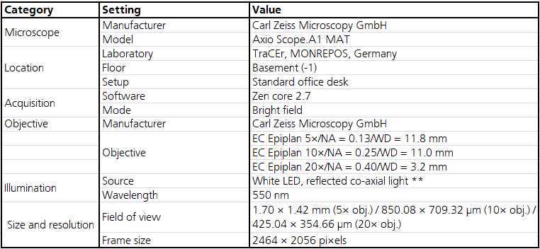
Acquisition settings

The qualitative use-wear analysis was done in a high-power approach by means of an upright light microscope (ZEISS Axio Scope.A1 MAT). The samples were studied using EC-Epiplan 5x/0.13, 10x/0.25 and 20x/0.40 objectives. Traces were documented as an EDF black and white image.

Equipment

Value	Label
Axio Scope.A1 MAT	NAME
Upright light microscope RL	TYPE
ZEISS	BRAND
-	SKU

Data acquisition: quantitative use-wear analysis

a) data acquisition on all 24 samples

First, the last state of the samples (after 2000 cutting strokes) was analysed. The samples were analysed for use-wear and within the use-wear, 3D surface data was acquired. Those exact three spots were analysed then also on the samples from before the first cycle (0 strokes), respectively.

Per sample, three surfaces per tool were acquired on the same use-wear area, but on non identical areas. Here, "surface" refers to the result of the acquisition, i.e. a 2.5 D image. The thee surfaces per sample are called "spot A", "spot B" and "spot C".

All surfaces were acquired on the flat side of the tools, i.e. side C (see section #1.7).

3surfaces +

× 24tools

x 2cycles

= 144surfaces

b) data acquisition on eight selected samples

In a second step, the same eight samples as described in step #7 b) were quantitatively analysed. The data acquisition was identical to #a). However, this time the samples were analysed before and after each cycle.

3surfaces +

× 8tools

x 5cycles

= 120surfaces

The majority of samples was studied as moulds (see step #5).

Acquisition settings

Equipment

Value	Label
LSM 800 MAT	NAME
Confocal microscope	TYPE
Carl Zeiss Microscopy	BRAND
-	SKU
Mounted on an Axio Imager.Z2 Vario	SPECIFICATIONS

Acquisition workflow

For each sample:

a) Calibrate coordinate system with 10× objective in WF mode, see:

b) Find location using 10× and 20× objectives in WF mode.

c) Acquire z-stack for topography with the 50×/0.95 objective in LSM mode (alternative: 20×/0.75 objective). Process z-stack for topography without noise cut. Save the result as a SUR surface (= "Spot A").

d) Repeat steps b) and c) two more times to measure non-identical spots within the same use-wear trace on the sample (= "Spot B" and "Spot C").

d) Acquire z-stack for black and white image at the same location with the same objective in WF mode and defining a 2×2 tile region (because the field of view is smaller in WF than in LSM mode, due to the 0.5× zoom). Process z-stack into EDF image and stitch it. Save the result as a PNG image.

e) Acquire z-stack for black and white image of the same location (entire use-wear) with the 10× objective and 20× in WF mode and defining a 2×2 / 2×1 tile region. Process z-stack into EDF image and stitch it. Save the result as a PNG image.

Processing for step #8.2d/e has been done in batch with a macro in ZEN blue.

Processing workflow quantitative use-wear analysis

The data acquired with the confocal microscope was processed in batch with templates in ConfoMap. For the analysed samples described in step #8a) the templates desribes as a), b) and d) have been used; for the samples described in step #8b) the templates a), b) c) and d) have been used instead.

Software

Value	Label
ConfoMap (MountainsMap Imaging Tophography)	NAME
Digital Surf, Besançon, France	DEVELOPER
https://www.digitalsurf.com/de/	LINK
ST 8.1.9286	VERSION

a) "mirroring template"

For the data acquired on moulds, an intital template was needed. Moulds always just display a mirrored version of the original surfaces. Therefore, the acquired surfaces needed to be mirrored in order to match the original surface again.

mirroring_FLT4-7.pdf

b) “aligning template”

A series of surfaces was built using the module "4D series" for ConfoMap. The coordinate system using the three beads (see step #1.7) repositioned the sample after each experimental cycle in order to acquire the same surface; nevertheless, this repositioning is not exact. This template allowed an exact repositioning and perfectly complements the coordinate system: the alignment in ConfoMap works only if the surfaces are similar enough and the more similar, the better. This way, the surfaces from identical samples measured after varying cycles within the experiment were compiled and aligned as precisely as possible.

aligning_FLT4-7.pdf

c) “resampling template”

A resampling in x and y on all 144 + 120 surfaces was performed, leading to an identical spacing. The template was necessary due to the different objectives used during data acquisition. After applying this template, all surfaces had the same size of 254.0 x 253.9 µm and 1198 x 1198 pixels.

resampling_FLT4-7.pdf

d) “processing template”

In a final step, the data was processed. The following procedure was performed:

I.   Levelling (least squares method by subtraction)

II.  Form removal (polynomial of degree3)

III. Outliers removal (maximum slope of 80°)

IV. Thresholding the surface between 0.1 and 99.9 % material ratio to remove the aberrant positive and negative         

      spikes 

V.  Applying a robust Gaussian low-pass S-filter (S1 nesting index = 0.425 µm, corresponding to about 5 pixels, end 

     effects managed) to remove noise

VI. Filling-in the non-measured points (NMP), VII.) Analysis: Calculation of 21 ISO 25178-2:2012 (International 

      Organization for Standardization, 2012) parameters, 3 furrow parameters, 3 texture direction parameters, 1 

      texture isotropy parameter and the scale-sensitive fractal analysis (SSFA) parameters epLsar, NewEplsar, Asfc, 

      Smfc, HAsfc9 and HAsfc81

processing _FLT4-7.pdf

The ConfoMap templates for each surface in MNT and PDF formats are available on Zenodo (10.5281/zenodo.6642970). This also includes all original and processed surfaces, as well as the results.

Data analysis

The processed data was statistically analysed with R.

Software

Value	Label
R Studio Desktop	NAME
The R Studio, Inc.	DEVELOPER
https://www.rstudio.com/products/RStudio/	LINK
1.1.463	VERSION

The analysis was separated into the two datasets:

a) all 24 samples from before and after 2000 strokes (called "analysis_before.after")

b) selected eight samples from all cycles (called "analysis_all.cylces")

Available in open access on Zenodo: 10.5281/zenodo.7229814

Results

Available in open access on Zenodo: 10.5281/zenodo.7229779