Quantitation of lower urinary tract afferents in 3D reconstruction of lumbosacral spinal cord sections

Each file should be a single image. Any z-steps need to be orthogonally projected into a single image for importation into TissueMaker (MBF Bioscience).

Prior to image importation, the series of images to be aligned need to be numbered in their anatomical order (typically rostrocaudal). TissueMaker acknowledges only the last digits in the file name. For example: Section001, Section002 etc. 

Open TissueMaker.

Under the heading 'Select slide image files', select ‘Add slide(s)’ located in the Workflow window (should open upon first starting the program), and select all the image files from their folder.

Click ‘Edit and order list’ to see the entire list of files chosen. Manual changes in their order can be made, or to allow the order of the list to be set by the digit assigned at the end of the file name, click ‘Sort list’.

Click ‘Next step’.

Unless whole slides and not individual sections were imaged, this option can be skipped, click ‘Next Step’.

Click ‘View Slides’.

Check the outline of each section, if editing is required click ‘Edit outlines’, otherwise click ‘Next slide’.

1. ‘Redetect and outline’ allows for the threshold of contouring to be altered, the most automated approach.
2. To remove specific imaging artefacts, outlines can be manually edited by clicking on the contour directly.
3. When contouring is finished on a section, the section order must be re-established, click ‘Start ordering’ and if only the section has a number one click ‘Done Ordering’.

When all section contours are satisfactory click ‘Next step’.

Click ‘Modify final section order’ to make any final changes.

Click ‘Next step’.

Select the mode of microscopy employed.

Selection of alignment mode determines processing time. The best balance between alignment and speed is achieved with ‘Align using shape’.

Each section will be presented superimposed upon the previous section. Use the controls to change orientation, flip sections and move them.

As the lumbosacral spinal cord gradually decreases inthickness, each subsequent section should be slightly smaller than the one that preceded it, if this is not the case, sections can be reordered by returning to the ‘Finalize section order’ step. If the order is altered, the ‘Align sections’ step will need to be repeated, however the‘Use parameters from previous alignment’ can be ticked to speed up the alignment process.

Upon review of all the sections, click ‘Next step’.

Choose the appropriate reconstruction output required for subsequent analysis:

• A ‘Single image stack’ produces an image stack (.jpx) that can only be opened using TissueMaker or Neurolucida 360 (MBF Bioscience).
• A ‘Series of image files’ produces individual aligned files that can then be converted into a single Imaris file (.ims) for use in Imaris.

The distance between spinal cord sections needs to be stipulated with the image processing in mind. 

For instance, as each image is a maximum intensity orthogonal projection of an image stack, the image thickness is no longer the thickness of the section. For example, if using a 1:2 series of 40 µm sections, the distance between image sections is 80μm rather than 40μm.

Select desired image resolution.

When ready, click ‘Save reconstruction’. When creating a .jpx image stack, this will be accompanied by a .xml file that will contain the metadata, ensure these files stay together.

Open Neurolucida 360, closing the 3D environment (which automatically opens with the program).

Open the image stack created in TissueMaker by other clicking and dragging the .xml file onto the open Neurolucida 360 window, or by going to 'File' and clicking 'Open file' to select the .xml file via the browser window.

The first section within the image stack should appear within the main window along with an outline (contour) of the entire section (created in Step 9). A few key tools will aid in the viewing of the stack:

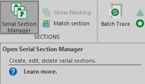
• In the 'Trace' tab, the 'Serial Section Manager' will open a small window wherein individual sections in the stack can be selected.
• In the 'Image' tab, the 'Image Adjustment' will enable the manipulation of brightness and contrast of the entire stack for each channel.
• In either of these tabs, the '3D Environment' will open a new window in which the entire stack will be reconstructed in 3D.

To define regions of interest on any given section, click on 'Contour'.

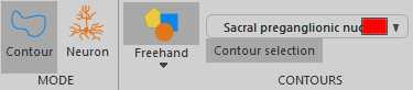
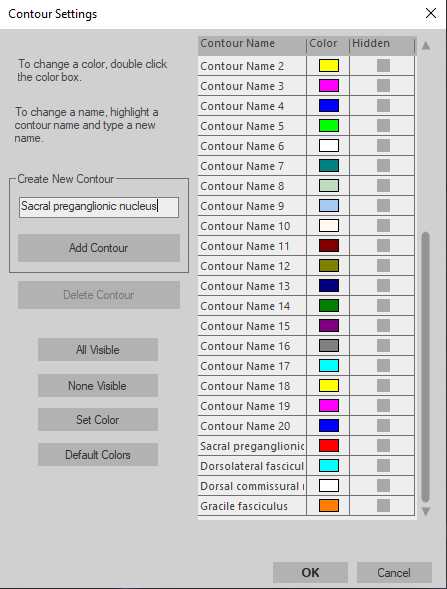
Select the relevant contour name from the drop down menu, or click on 'Contour selection' in order to choose from a larger list or create a new contour that is not available.

With the correct contour selected, begin drawing the contour using the 'Freehand' method by clicking to start the contour and continue clicking to add vertices to the contour. To finish the contour, right click and select 'Close Contour'. Alternative contour drawing methods can be chosen, including circular and rectangular contours.

Continue adding contours for regions in all the relevant sections, using the Serial Section Manager to navigate between sections.

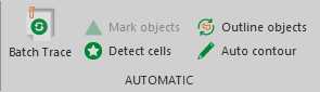
To begin the detection of cholera toxin B-labelled afferents, click on 'Detect cells' in the Trace tab of Neurolucida 360. This should bring up the Cell Detection Workflow.

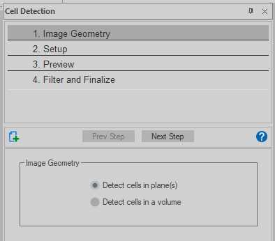
Under Step 1 of the workflow, select 'Detect cells in plane(s)' because we are using a dataset of serial sections.

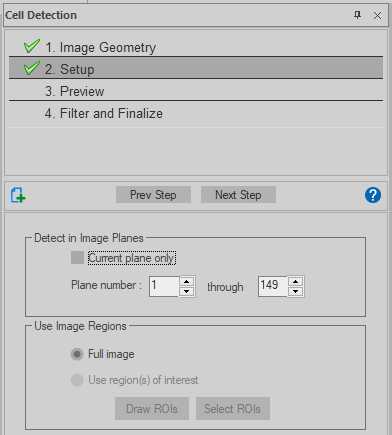
Under Step 2 of the workflow, deselect 'Current plane only' ensuring all the planes (ie. sections) are included. Select 'Full Image'. This is because the Cell Detection workflow does not work for image regions when part of an image stack.

Under Step 3 of the workflow, select the following:

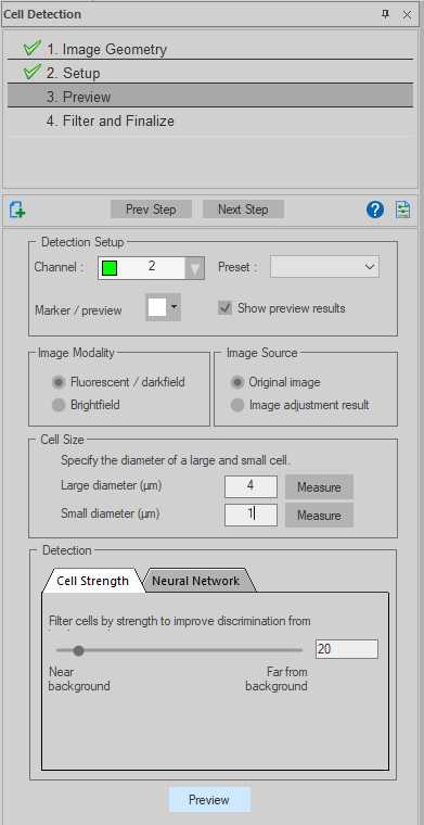
Select the channel in which cholera toxin-B was labelled (in the case of our datasets, Channel 2 was Cy3).

Select 'Fluorescent' under Image Modality.

Select 'Original image' under Image Source.

Input the diameter size for the largest and smallest cells to be detected under Parameters. The 'Measure' button, on clicked, will change the cursor to a circle. The diameter of this circle can be altered by scrolling the mouse wheel, overlay this onto examples of the smallest and largest boutons to find diameters. Left click to save the diameter value to the selected Parameter field. In the case of our datasets, a maximum of 4 μm and a minimum of 1 μm was chosen.

Click 'Preview' with 'Run preview detection on displayed image' selected. Use the slider to optimize the detection of cholera toxin B versus background. When satisfied, go to next step.

Under Step 4 of the workflow, click 'Detect'. A progress bar should appear indicating the % of all cells detected. On large image stacks (50+ sections) this can take a while, do not attempt to interact with Neurolucida 360 until detection is complete.

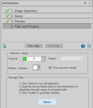
Once detection is complete, a histogram will appear indicating all the 'cells', and what percentage have been detected according to thresholding parameters set in step 31.5. Additional thresholding can be done here. When satisfied, select an appropriate marker from the drop-down menu and click 'Finalize'. Markers will now be assigned to each detected cell (in this case cholera toxin B-labelled boutons) throughout the image stack.

Save the file and close Neurolucida 360.

Open Neurolucida Explorer, and with it open the .xml file associated with the TissueMaker image stack. The .xml file contains the segmentation data.

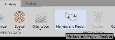
Click on 'Markers and Counters' under the 'Analyze' tab.

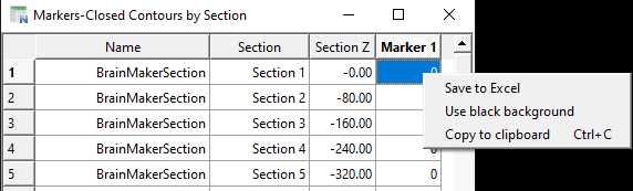
A new window will open for 'Markers and Region Analyses'. On the left-hand side select the 'Markers and Contours' tab and from the offering select 'Markers in Closed Contours by Section'.

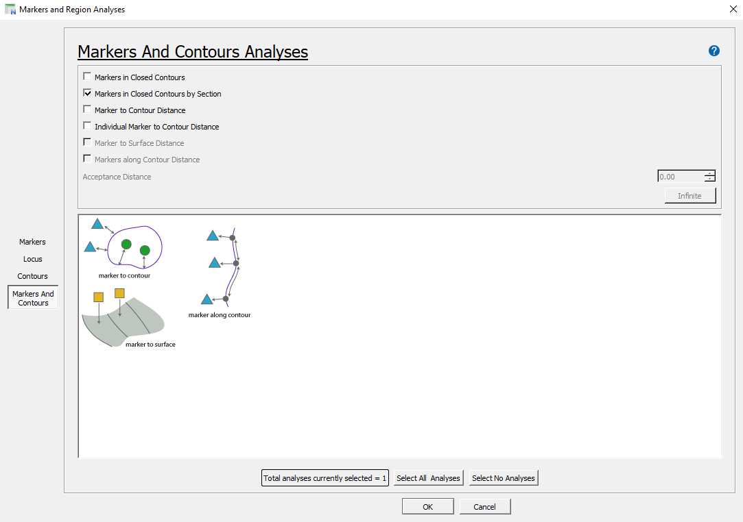
The number of markers (ie. cholera toxin B-labelled boutons) per section within each of the regions will then be displayed in table form in a new window. To export this, right click anywhere on the table and either click 'Save to Excel' to produce a .csv, or 'Copy to clipboard' to paste into a prepared Excel document.