Quality control assessment for microbial genomes: GalaxyTrakr MicroRunQC workflow
Ruth Timme, Maria Balkey, William Wolfgang, Errol Strain, Robyn Randolph, Sai Laxmi Gubbala Venkata
Disclaimer
Please note that this protocol is public domain, which supersedes the CC-BY license default used by protocols.io.
Abstract
PURPOSE: Step-by-step instructions for checking WGS sequence quality. The MicroRunQC workflow, implemented in a custom Galaxy instance, will produce quality assessments for raw reads (Illumina paired-end fastq files) and draft de novo assemblies, along with reporting the sequence type for each isolate. This workflow will work on most microbial pathogens, so we advise laboratories to upload their entire MiSeq/NextSeq run through this workflow.
SCOPE: This protocol covers the following tasks:
-
set up an account in GalaxyTrakr
-
Create a new history/workspace
-
Upload data
-
Execute the MicroRunQC workflow
-
Interpret the results
V3: updated with Cronobacter thresholds
Before start
Steps
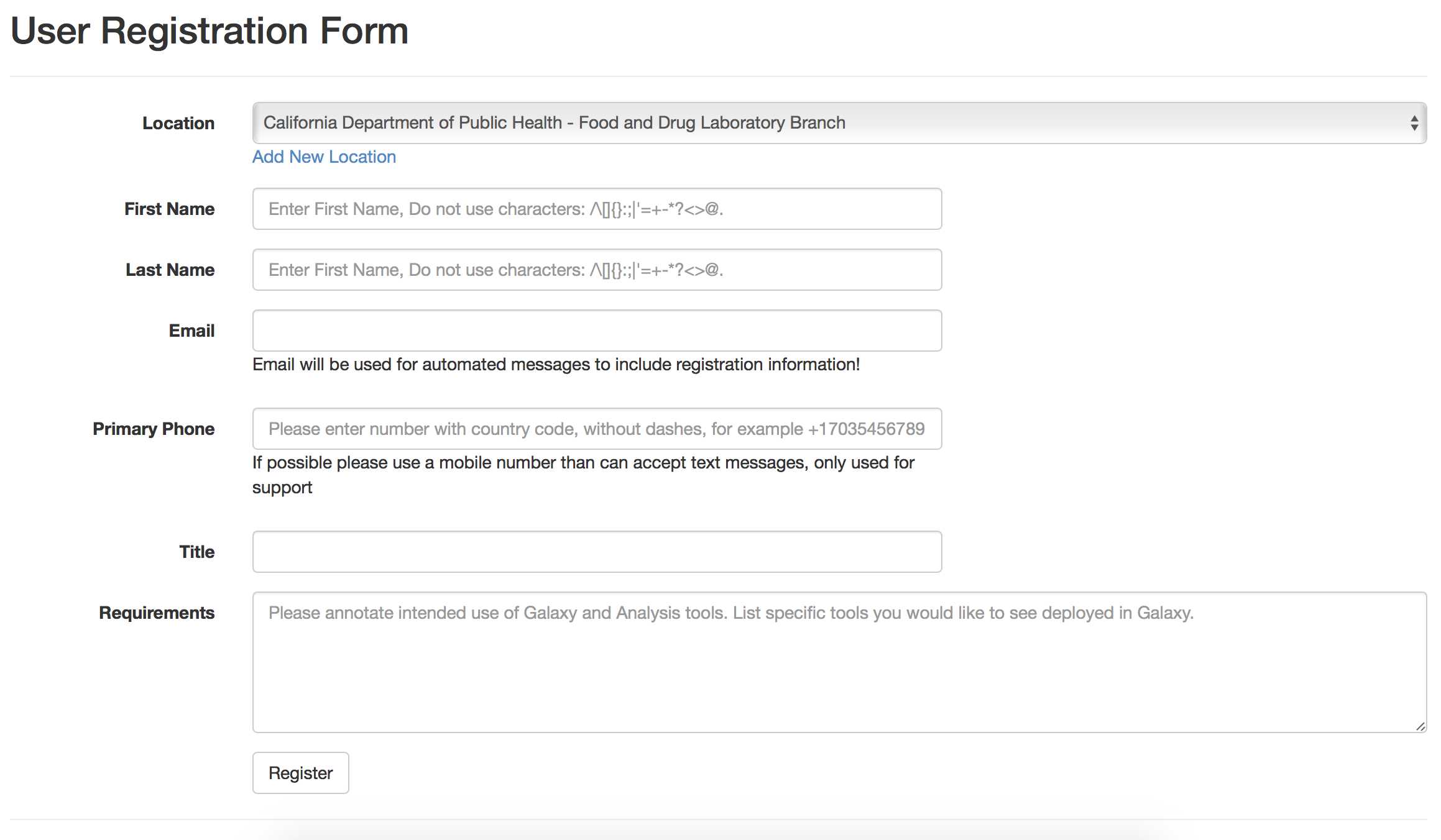
Account set up
Create a GalaxyTrakr account here: https://account.galaxytrakr.org/Account/Register
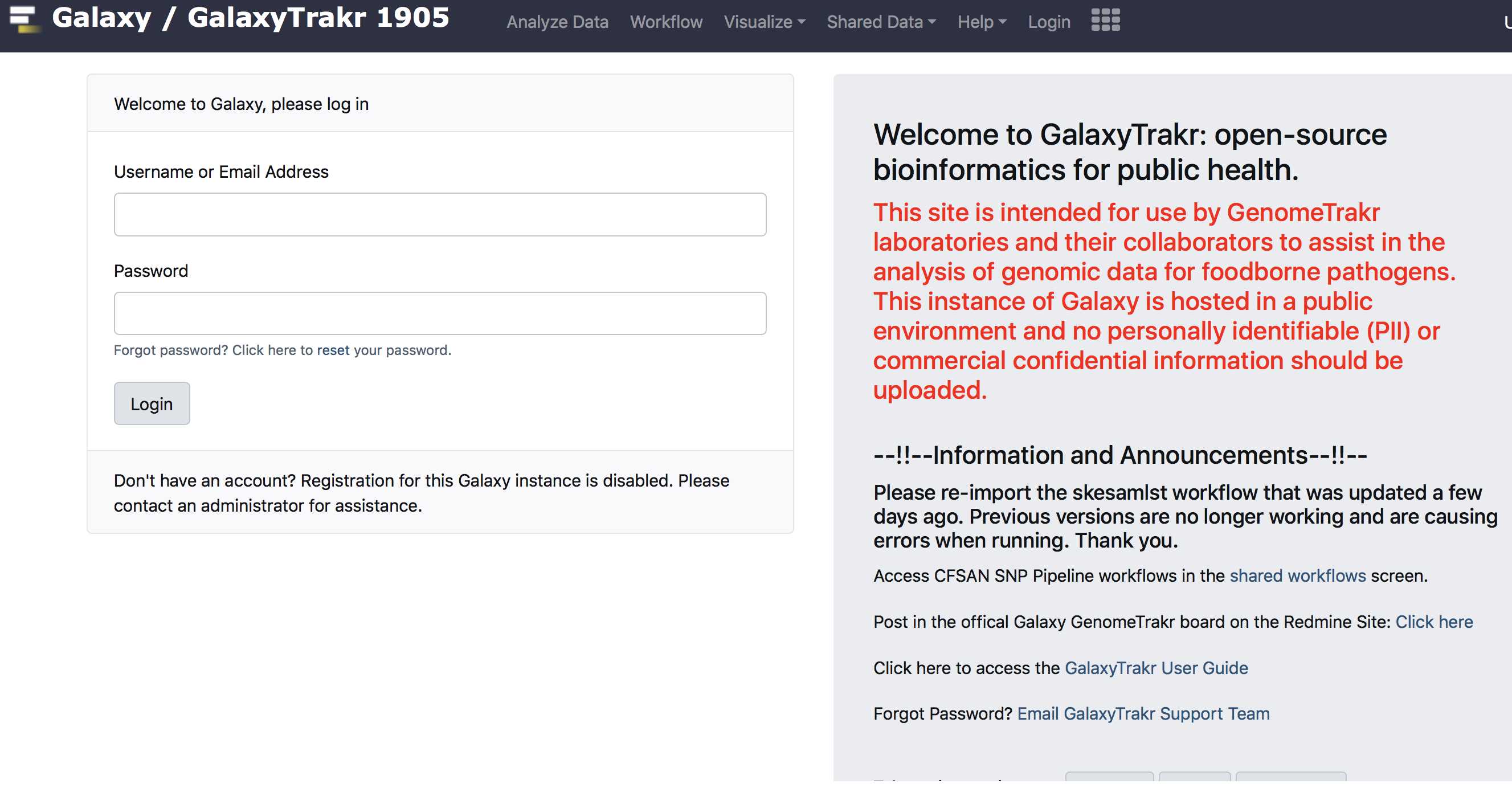
Log into your GalaxyTrakr account: https://galaxytrakr.org
Create a new history
Create a new history.
We recommend creating a new history for each new MiSeq Run and including the flow-cell ID and date in the history name.
Save your MicroRunQC output here and any other relevant analyses, like serotyping, or AMR detection.
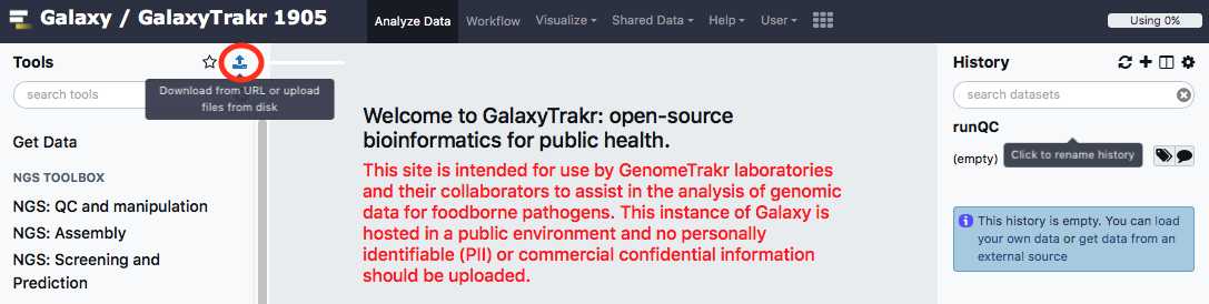
After all the analysis output from this run is saved to your internal data network or computer, older history's should be purged/deleted so as not to occupy the limited storage space in your account. In some cases it may be useful to save, for a limited time, multiple histories or to run analyses concurrently in multiple histories. In these cases you need to pay attention to your % usage bar (shows % used of allocated storage space) in the upper right corner of the GalaxyTrakr page. If you need additional space you can contact galaxytrakrsupport@fda.hhs.gov and request additional storage.
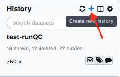
Click on the + icon in the upper right History panel
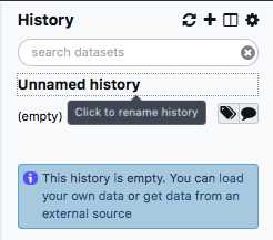
Name your new History by clicking on the “Unnamed history”, type in desired name and hit enter. We recommend including the run cell ID and the date the run was started.
Upload data
This section will describe the process for uploading raw fastq files into your active History panel. After the files have been uploaded they will stay in your account until they are deleted.
Click on the upload/download icon on the top of the left web page to start an upload process.
Select "Type (set all):auto-detect." Choose local file button and navigate to the desired fastq files, then click "start" to upload files. These files should be paired (two per sample/isolate).
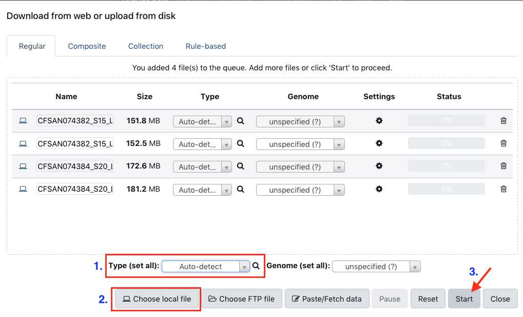
As the file uploads complete, each row will turn green. Samples in yellow are still in process.
You have just upload a set of forward and reverse reads. For further analysis these files need to be paired properly so the platform knows which R1 and R2 files go with each sample/isolate. GalaxyTrakr does this by creating a List of Dataset Pairs.
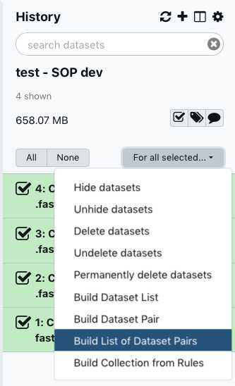
Within your newly created History panel, click the "check box," then select all the files you just uploaded by clicking "All" or by individually selecting the ones you want to pair.

Click "For all selected" and choose "Build List of Dataset Pairs"
A new window will open to help you pair the fastq files properly. Note how your paired reads are named (_R1 and _R2 in the example above)
Select Clear filters , then click Auto-pair.
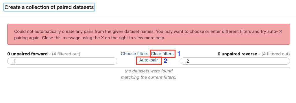
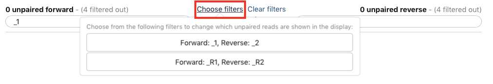
Alternatively, instead of autopairing you can click "choose filters" and select the appropriate filter for the pairing:
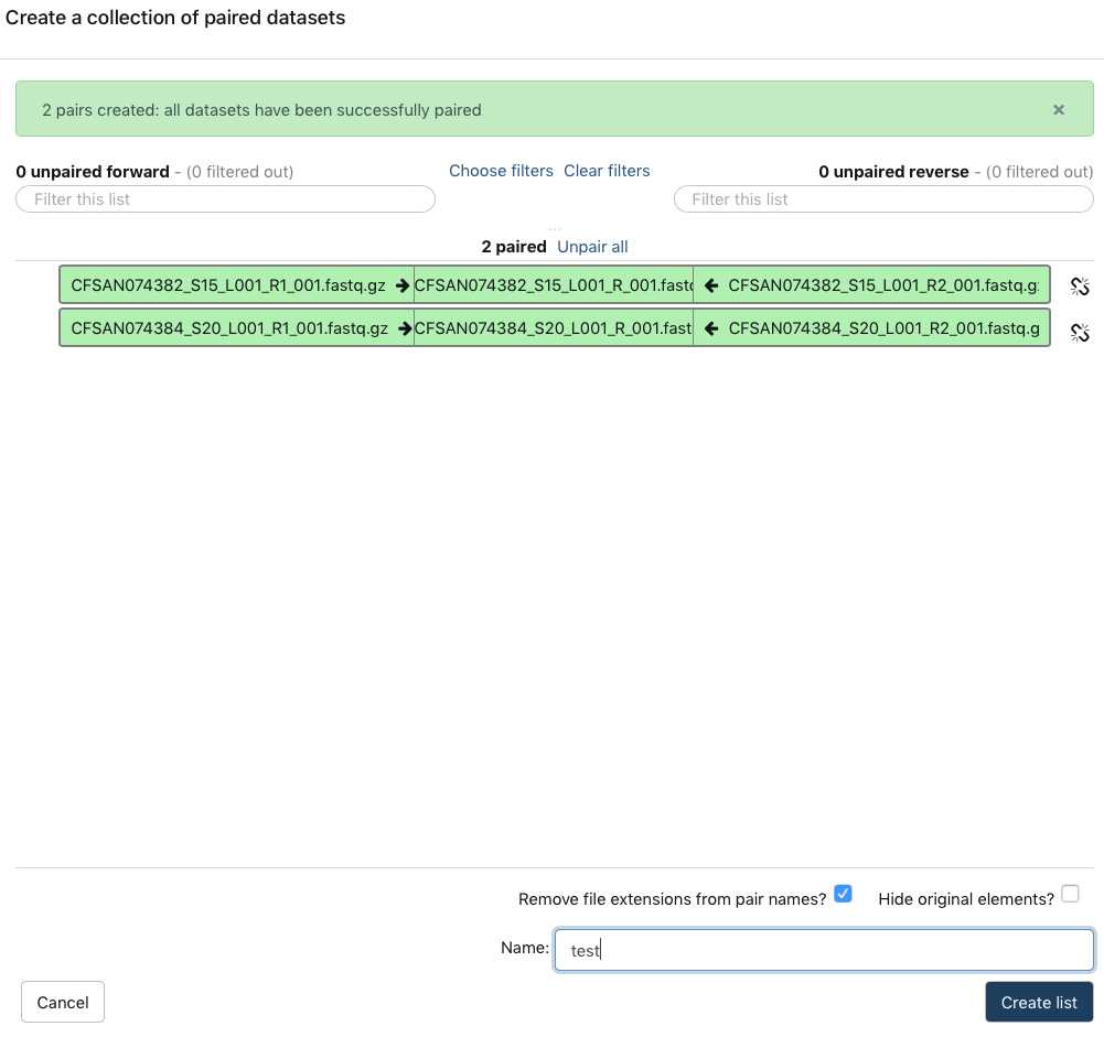
Paired reads will pair in the middle column and turn green.
Name your dataset: Example, "pairedSet-
Click Create list.
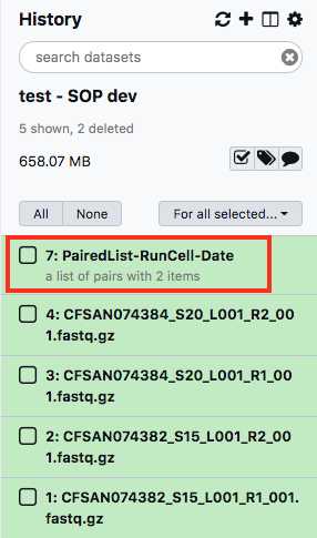
This paired dataset will now be available for analysis in your history panel. You can run multiple analyses on the same dataset in a history rather than upload the same sequence data to a new history to perform additional analyses. This will help you use your allocated storage space efficiently.
Run the MicroRunQC workflow
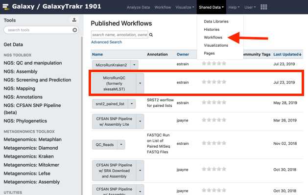
Add the MicroRunQC workflow to your own "workflows" panel. You only have to do this step once for each new workflow you need.
Navigate to the “Shared Data" drop down menu, choose workflows and from the MicroRunQC drop down menu select import.
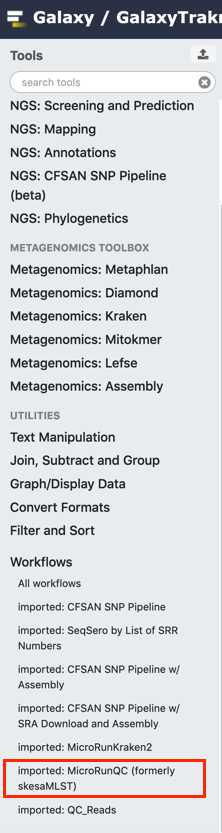
To see the new workflow in your “Workflows” tools panel on the left, open the Workflow tab and check “show in tools panel” for the workflow of interest.
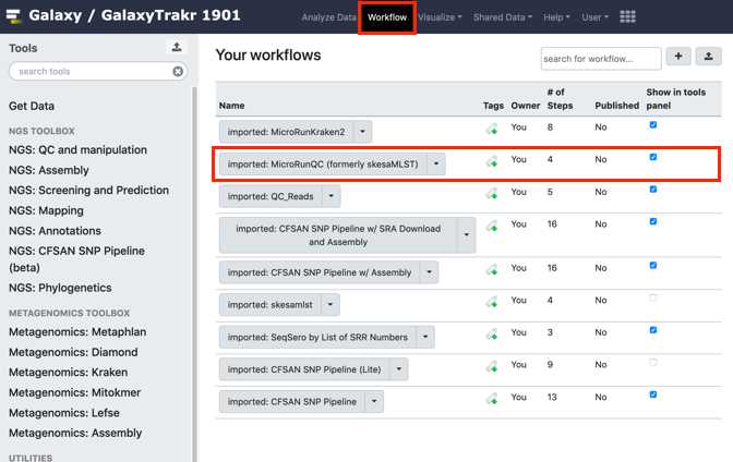
From the workflow menus select MicroRunQC
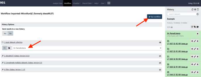
Select paired list dataset you created earlier.
Click Run Workflow. This can take some time depending on the number of samples you are analyzing. If you choose to you can log out of GalaxyTrakr and log back in at a later time to see if the job is completed.
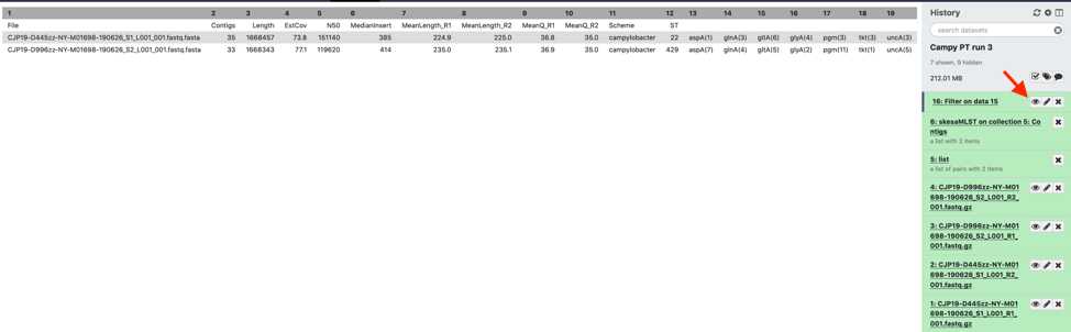
Upon completion of the pipeline all tiles in the history bar will be green.
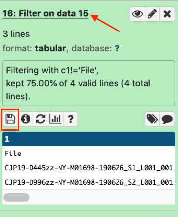
In the “Filter on Data” tile click on the “Eye” icon to view the output in the GalaxyTrakr window.
Interpret the results
Download and interpret the results:
Click “Filter on data” and then the floppy disc icon. The tabular file can be opened in a text reader or converted to a format that can be opened on excel.
The MicroRunQC output file includes the following metrics:
Parameter | A | B | C | | --- | --- | --- | | Parameter | Input | Description | | Contigs | Assembly | Number of contigs in the de-novo SKESA assembly. Contigs smaller than 200 base-pairs (bp) are not counted. | | Length | Assembly | Total length of all contigs > 200bp. This should approximate the size of the genome for the target organism. | | EstCov | Assembly | Mean coverage for contigs in the SKESA assembly. | | N50 | Assembly | Sequence length of the shortest contig at 50% of the total genome length | | MedianInsert | Read | Distance between forward and reverse reads. Calculated by mapping reads to SKESA assembly using bwa. | | MeanLength_R1 | Read | Mean length of forward read | | MeanLength_R2 | Read | Mean length of reverse read | | MeanQ_R1 | Read | Mean Q-score of forward read | | MeanQ_R2 | Read | Mean Q-score of reverse read | | Scheme | Assembly | PubMLST (pubmlst.org) database scheme (e.g. senterica for Salmonella enterica) | | ST | Assembly | Sequence Type | | Loci | Assembly | gene (allele number) – for example aroC(118) |
MicroRunQC output table headers. This table lists the summary metrics for sequence quality, number of contigs, and estimated genome size, along with other common metrics for reads (Median Insert Size and Mean Length) and assemblies (N50). Additionally, if the Multi-Locus Sequence Type (MLST) for the isolate is available from pubmlst, the workflow also reports Sequence Type (ST) and the associated alleles. Input Description Contigs Assembly Number of contigs in the de-novo SKESA assembly. Contigs smaller than 200 base-pairs (bp) are not counted. Length Assembly Total length of all contigs > 200bp. This should approximate the size of the genome for the target organism. EstCov Assembly Mean coverage for contigs in the SKESA assembly. N50 Assembly Sequence length of the shortest contig at 50% of the total genome length MedianInsert Read Distance between forward and reverse reads. Calculated by mapping reads to SKESA assembly using bwa. MeanLength_R1 Read Mean length of forward read MeanLength_R2 Read Mean length of reverse read MeanQ_R1 Read Mean Q-score of forward read MeanQ_R2 Read Mean Q-score of reverse read Scheme Assembly PubMLST (pubmlst.org) database scheme (e.g. senterica for Salmonella enterica) ST Assembly Sequence Type Loci Assembly gene (allele number) – for example aroC(118)
**This output should be saved either to your LIMS or to a spreadsheet linked to the sequencing run and samples.
Example output for 4 Listeria samples run through the MicroRunQC workflow:
| A | B | C | D | E | F | G | H | I | J | K | L | M | N | O | P | Q | R | S |
|---|---|---|---|---|---|---|---|---|---|---|---|---|---|---|---|---|---|---|
| File name | Contigs | Length | EstCov | N50 | MedianInsert | MeanLength_R1 | MeanLength_R2 | MeanQ_R1 | MeanQ_R2 | Scheme | ST | |||||||
| FSL-R9-8346 | 14 | 2876874 | 87.8 | 512255 | 408 | 147.6 | 147.7 | 33.1 | 32.7 | lmonocytogenes | 389 | abcZ(52) | bglA(1) | cat(12) | dapE(71) | dat(2) | ldh(1) | lhkA(5) |
| FSL-R9-8348 | 11 | 2832172 | 84.2 | 1464158 | 388 | 147.9 | 147.9 | 33.2 | 32.9 | lmonocytogenes | 795 | abcZ(7) | bglA(10) | cat(18) | dapE(6) | dat(5) | ldh(7) | lhkA(1) |
| FSL-R9-8350 | 14 | 2884629 | 64.2 | 450082 | 390 | 147.2 | 147.2 | 33.1 | 32.7 | lmonocytogenes | 37 | abcZ(5) | bglA(7) | cat(3) | dapE(5) | dat(1) | ldh(8) | lhkA(6) |
| FSL-R9-8352 | 12 | 2902520 | 85.9 | 1460419 | 390 | 148.1 | 148.2 | 33.1 | 32.8 | lmonocytogenes | 391 | abcZ(7) | bglA(6) | cat(62) | dapE(28) | dat(5) | ldh(2) | lhkA(1) |
Spreadsheet showing example output for 5 Listeria monocytogenes samples from a NextSeq sequencing run.
Quality control threshold guidelines for the GenomeTrakr surveillance network. These are also relevant for NARMS and VetLIRN contributors.
*MicroRunQC users should follow threshold guidelines established by their respective surveillance coordinating body(s).
| A | B | C | D | E | F | G | H |
|---|---|---|---|---|---|---|---|
| Quality metric | Salmonella | Listeria | E. coli | Shigella | Campylobacter | Vibrio para. | Cronobacter |
| Average read quality Q score for R1 and R2 | >=30 | >=30 | >=30 | >=30 | >=30 | >=30 | >=30 |
| Average coverage | >=30X | >=20X | >=40X | >=40X | >=20X | >=40X | >=20X |
| De novo assembly: Seq. length (Mbp) | ~4.3-5.2 | ~2.7-3.2 | ~4.5-5.9 | ~4.0-5.0 | ~1.5-1.9 | ~4.8-5.5 | ~4-5 |
| De novo assembly: no. contigs | <=300 | <=300 | <=500 | <=650 | <=300 | <=300 | <=500 |
