Bioinformatics Analysis of Estrogen-Responsive Genes

Adam E. Handel

Published: 2021-09-03 DOI: 10.17504/protocols.io.bnw9mfh6

Abstract

Estrogen is a steroid hormone that plays critical roles in a myriad of intracellular pathways. The expression of many genes is regulated through the steroid hormone receptors ESR1 and ESR2 . These bind to DNA and modulate the expression of target genes. Identification of estrogen target genes is greatly facilitated by the use of transcriptomic methods, such as RNA-seq and expression microarrays, and chromatin immunoprecipitation with massively parallel sequencing (ChIP-seq). Combining transcriptomic and ChIP-seq data enables a distinction to be drawn between direct and indirect estrogen target genes. This chapter discusses some methods of identifying estrogen target genes that do not require any expertise in programming languages or complex bioinformatics.

Attachments

Handel2016_Protocol_BioinformaticsAnalysisOfEstrog.pdf

Steps

3.1 The Genomic HyperBrowser

Prepare ChIP-seq and transciptomic datasets for upload. ChIP-seq files should be a set of tab-delimited genomic coordinates corresponding to each peak in the format:

Chromosome Start Stop

Transcriptomic files should be a list of differentially expressed genes (DEGs) as ENSEMBL IDs ( see Note 1 for methods for converting between different forms of gene ID). The datasets used for this demonstration are the ESR1 binding site data (actually ChIP-chip data) from Hurtado and colleagues and transcriptomic data from Hah and colleagues (thresholded at q < 0.05) [6, 19].

Note

Note 1: Converting between different gene IDs : There are multiple ways of converting between different forms of gene ID (e.g., gene symbol, RefSeq, ENSEMBL). One simple way is to use the Table Browser function in UCSC Genome Browser (Converting between different gene IDs: There are multiple ways of converting between different forms of gene ID (e.g., gene symbol, RefSeq, ENSEMBL). One simple way is to use the Table Browser function in UCSC Genome Browser (http://genome.ucsc.edu/) (Fig.6) [23]. It is possible to convert gene IDs between multiple types of gene ID using sequential conversions.) (Fig.6) [23]. It is possible to convert gene IDs between multiple types of gene ID using sequential conversions.

Fig. 6Convert gene IDs from one form to another. Select the required clade, the species and the genome build. Select the “Genes and Gene Predictions” group of tables, the appropriate track (e.g., Ensembl genes), the desired table (this will be one that maps the gene ID one has to the gene ID one requires), paste the list of gene IDs (this will be checked for unknown IDs by the system), select that output should be “selected fields from primary and related tables,” and then select “get output.” On the resulting screen it is possible to select the desired fields to obtain the gene ID of interest

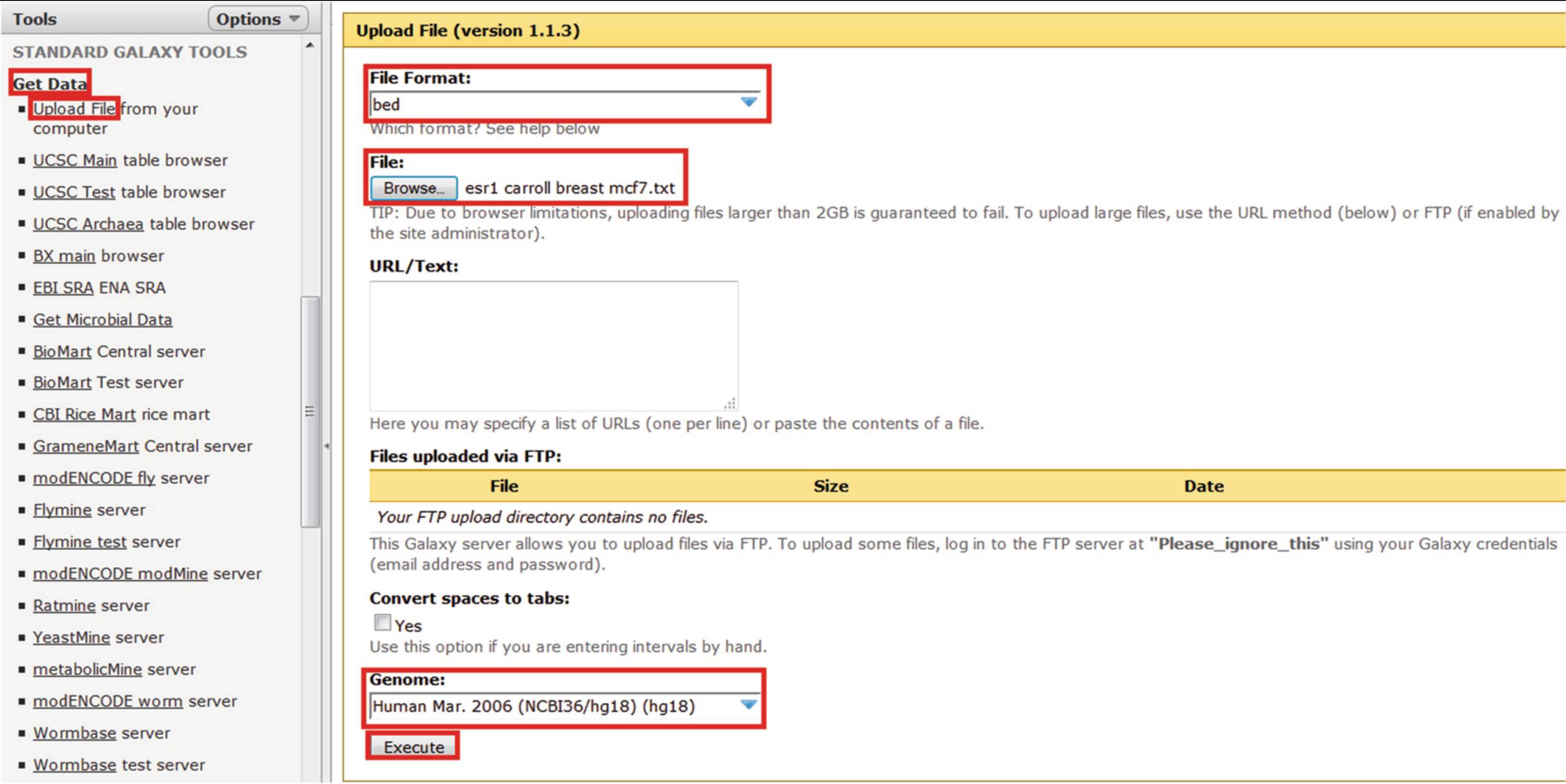
Firstly upload the ChIP-seq data as shown in Fig. 1.

Fig. 1Uploading files to the Galaxy/Genomic HyperBrowser server. Select “Get Data > Upload files,” select the correct file type (in this case “bed” for ChIP-seq data or “txt” for transcriptomic data), select the file location using the “browse” button, select the correct genome build, and then select “Execute”

Next use “Generate Tracks > Generate segment track from gene IDs” to obtain genomic intervals from the ENSEMBL gene IDs of DEGs. These should be uploaded into the tool as a series of comma-separated values as shown by the demo data. If necessary genomic intervals can be lifted from one genome build to another by the “Lift-Over > Convert genomic coordinates” tool.

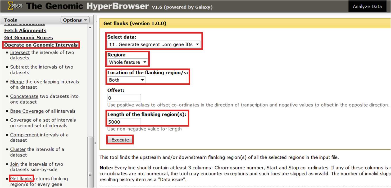
Use “Operate on Genomic Intervals > Get flanks” to extend gene regions by a pre-specified number of bases in each direction (Fig. 2). A suitable distance might be 5 kb, which is analogous to the upstream region extension in the gene ontology tool GREAT [20].

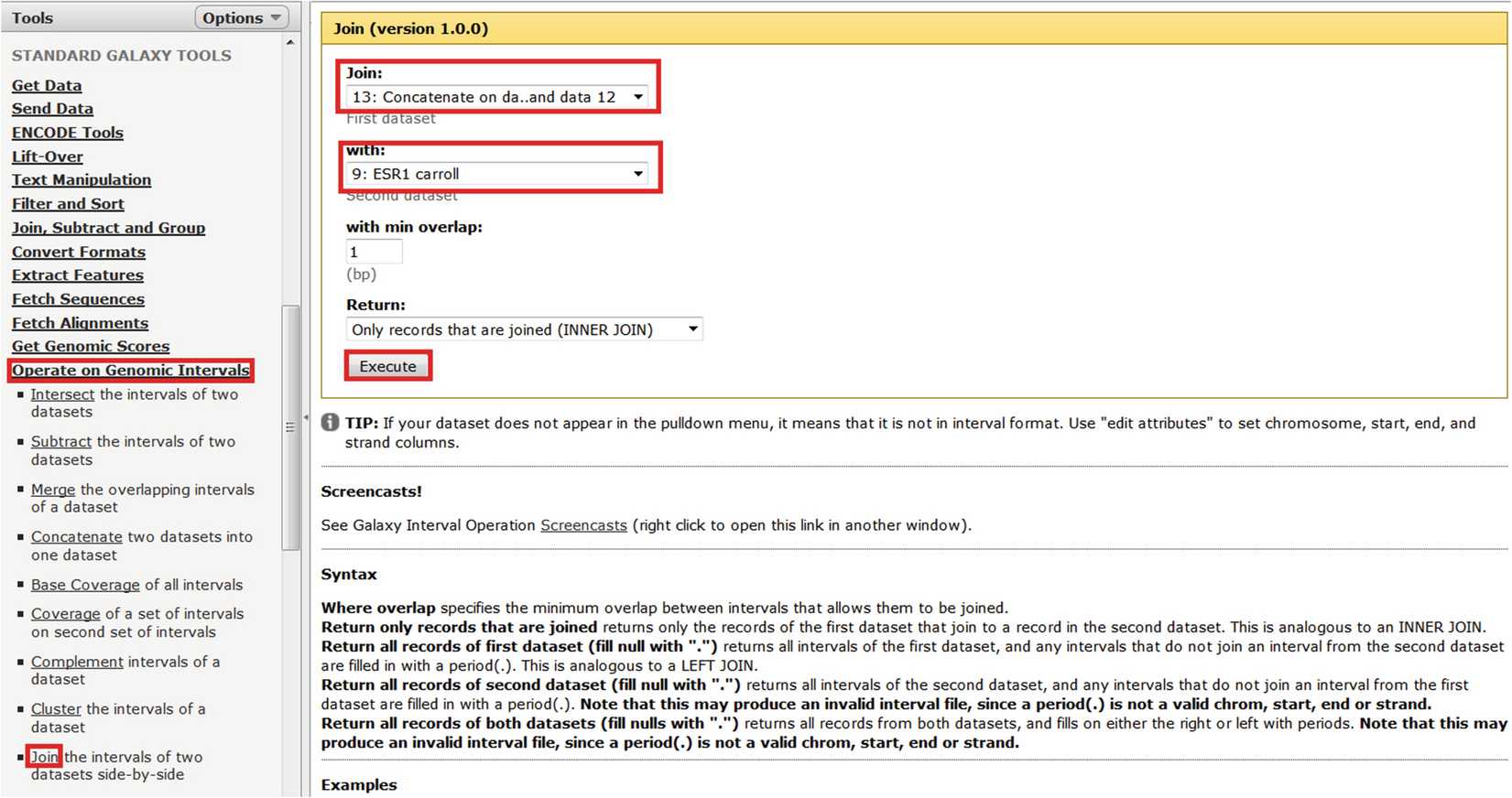
Fig. 2Generating a track of regions flanking differentially expressed genes. Select “Operate on Genomic Intervals > Get flanks,” select the desired track, select the subset of the region to flank (in this case “whole region”), select whether to extend flank from the upstream, downstream or both sides of regions, decide on the length of flanking regions, and then select “Execute”

The original intervals and flanking regions should then be concatenated into a single track using “Operate on Genomic Intervals > Concatenate” and then merged with “Operate on Genomic Intervals > Merge.”

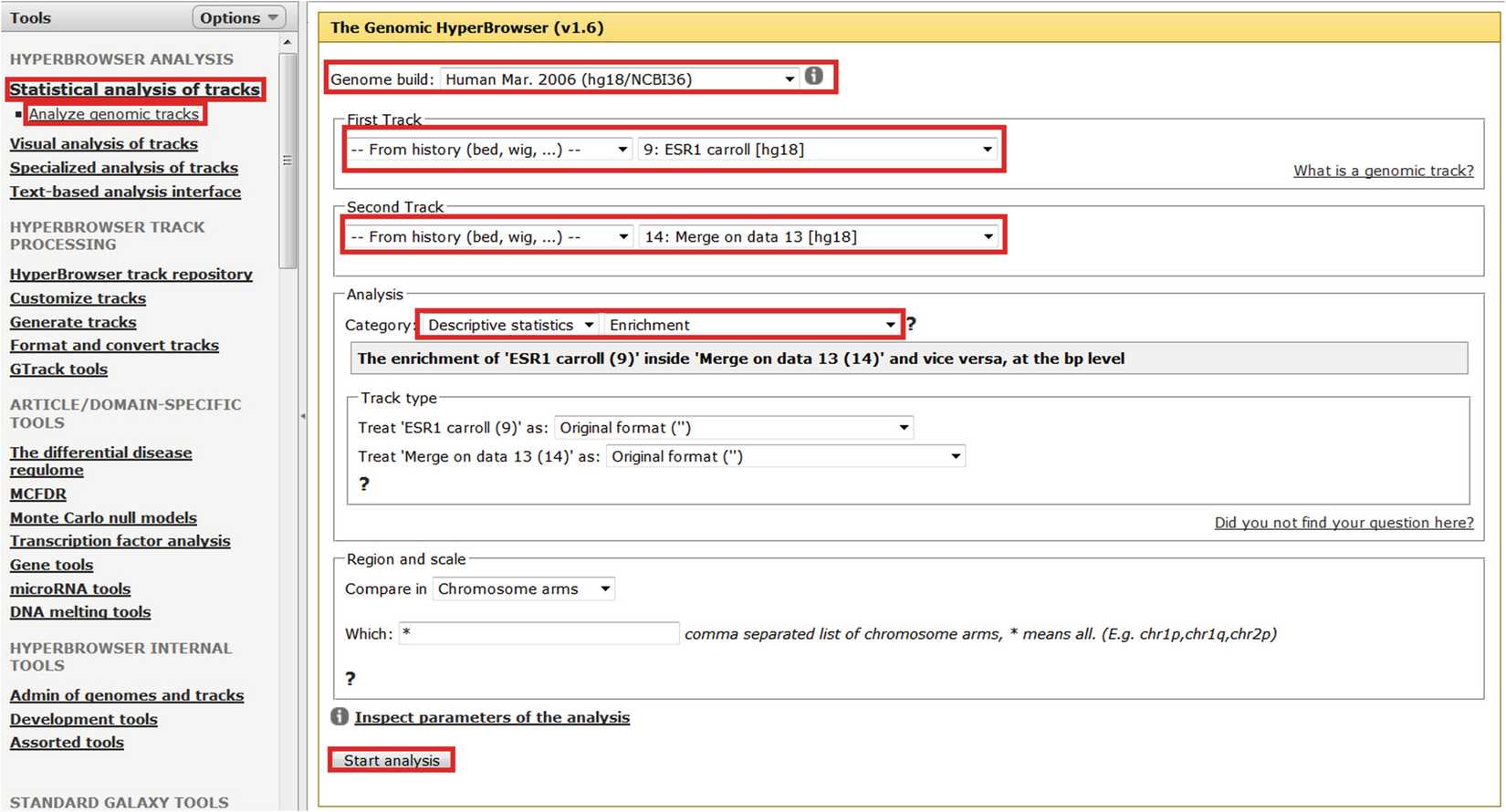
An important sanity check is to ensure that estrogen receptor binding is enriched near estrogen DEGs. The Genomic HyperBrowser allows one to calculate the enrichment of estrogen receptor-binding sites with the intervals generated above (i.e., within 5 kb of estrogen DEGs). Figure 3 illustrates this process. It is possible to use the Genomic HyperBrowser to calculate an empirical p-value for this overlap using the same tab as for enrichment analysis but selecting “Category: Hypothesis testing,” “Overlap?,” a suitable null model (e.g., “Preserve segments (T2), segment lengths and inter-segment gaps (T1); randomize positions (T1) (MC)”) and the number of permutations (e.g., for publication quality p-values ~10,000 permutations would be recommended). The region and scale tab is also important as this determines in which areas of the genome randomized tracks can fall. Leaving it at its default value (all chromosome arms) is adequate for the current sanity check. There is significant overlap between ESR1-binding sites and estrogen DEGs (2.14-fold, p < 10−4), which suggests that there are likely to be plausible direct estrogen targets amongst the transcriptomic dataset. Note that analyses are only conducted on bed files, and so if the track of interest is not offered by the Genomic HyperBrowser as a potential track for analysis then edit that track to ensure that the track type is “bed.”

Fig. 3Performing enrichment analysis. Select “Statistical analysis of tracks > Analyze genomic tracks,” select the genome build, select that each track for analysis will be from your history and then select the appropriate track, select “Descriptive statistics,” select “Enrichment,” and then select “Start analysis”

Identifying potential direct estrogen targets is simply a matter of joining estrogen DEGs (±5 kb) to ESR1-binding sites (Fig. 4).

Fig. 4Joining two tracks side by side. Select “Operate on Genomic Intervals > Join,” select the required tracks, and then select “Execute”

The resultant output can be pasted into a spreadsheet program and filtered to obtain unique gene IDs and their respective ESR1-binding sites.

3.2 BETA

10.

Register for Galaxy/Cistrome (http://cistrome.org/ap/). This tool integrates transcription factor-binding sites with the degree of differential gene expression to predict high-confidence direct targets.

11.

Prepare ChIP-seq and transcriptomic data for upload. Again, the ChIP-seq data should be a tab-delimited file in the format:

Chromosome Start Stop

RNA-seq data can either be directly uploaded as Cuffdiff or LIMMA output [21, 22] or formatted as a tab-delimited file with columns corresponding to gene ID, direction of change (e.g., T-score ) and significance (e.g., FDR). Ensure that all data are present as text (gene ID) or numerical data. Some spreadsheet programs can format data in ways that will cause BETA to crash (e.g., substituting dates for numerical values).

12.

Start the BETA tool running after selecting the appropriate parameters (Fig. 5). The BETA tool is available through “Integrative Analysis > BETA-plus: Binding and Expression Target prediction and motif analysis.” For an initial analysis, it is recommended to leave as many settings at their default values as possible. Subsequently these can be altered to test how robust the results are to changes in, for example, the distance threshold of ESR1-binding sites to DEGs.

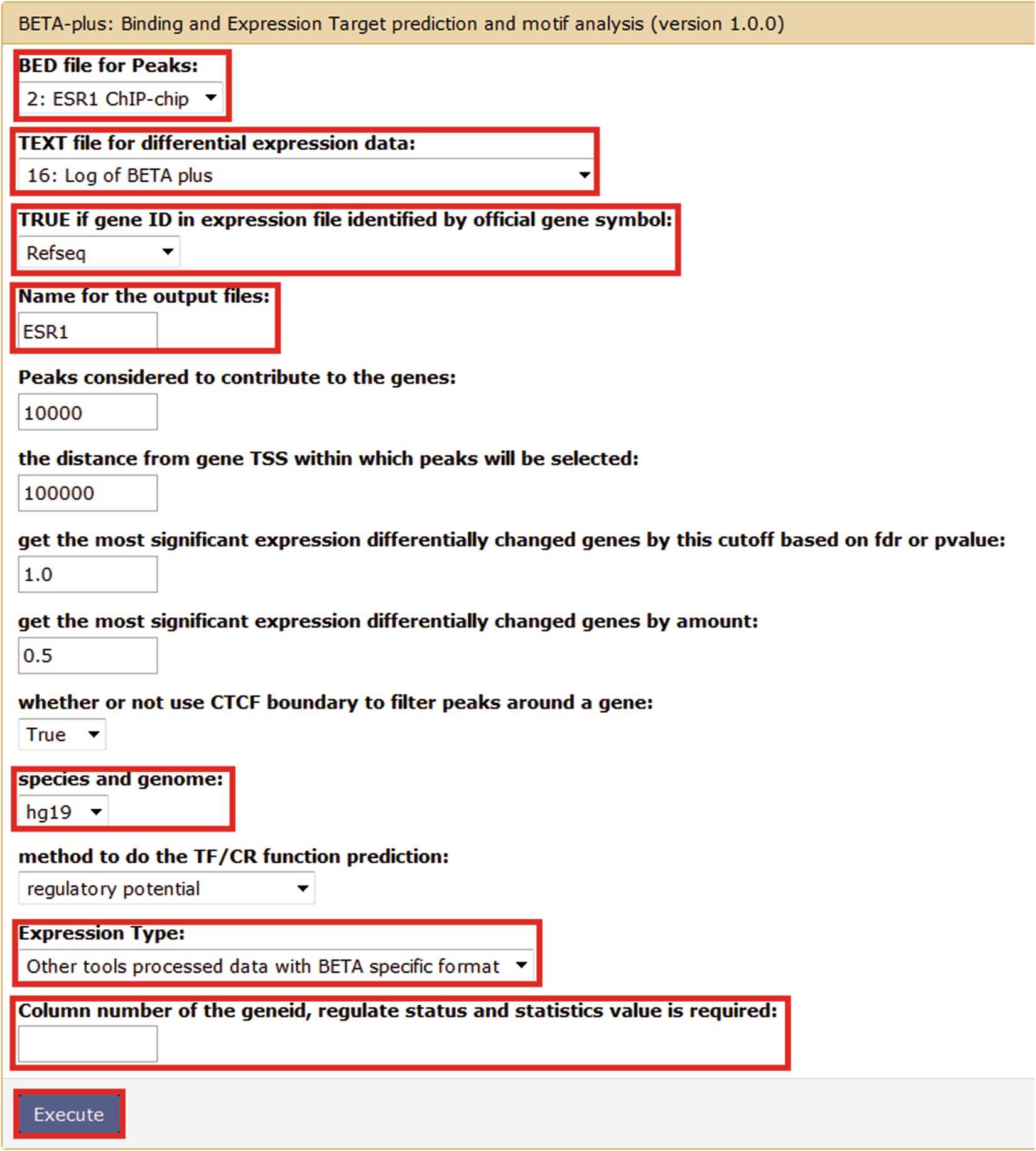
Fig. 5Performing BETA-plus analysis. Select the track containing the ChIP-seq data, select the track containing the transcriptomic data, select the type of gene ID used (RefSeq or gene symbol), input the prefix for output files, select the genome build, select the type of transcriptomic data (i.e., the format of the track selected earlier), if the transcriptomic data is in a custom format insert a comma-separated list of numbers referencing which column is the gene ID, the direction of expression change and the significance measure (e.g., if this was a track with three columns, the first of which was the gene ID, the second of which was the log2fold change and the third of which was the FDR, this would be 1,2,3). Finally select “Execute”

13.

The output files then produce direct target predictions. These are described below:

BETA functional prediction on ESR1 ChIP-chip: A graph showing the relationship between functional rank and the number of direct targets and an associated p-value for upor downregulated genes.
BETA direct targets prediction on up regulated genes: A table of up-regulated gene targets detailing the rank product score (derived from the significance score provided in the transcriptomic dataset).
BETA direct targets prediction on down regulated genes: A table of downregulated gene targets detailing the rank product score (derived from the significance score provided in the transcriptomic dataset).
Uptarget associated peaks: A list of peaks with the associated up-regulated gene target, the distance to the target gene, and a functional score.
Downtarget associated peaks: A list of peaks with the associated downregulated gene target, the distance to the target gene, and a functional score.
Motif analysis on target regions: An html output file detailing top motifs detected for multiple comparisons along with associated statistical scores.
A series of detailed motif analysis outputs: The statistical data for the above file.
Log of BETA plus: This details the input parameters and any errors encountered during the course of the analysis.