BTI mobile plant phenotyping system: Image analysis protocol
Li'ang Yu, Magdalena M Julkowska
Abstract
This protocol is a part of BTI mobile plant phenotyping system (https://github.com/Leon-Yu0320/BTI-Plant-phenotyping). In this part, we'll introduce using jupyter book as an interactive user-friendly interface to set appropriate parameters for image analysis by PlantCV.
Steps
Package installation
Installation of packages required for analyiss
Jupyter notebook and plantCV are reuqired for analysis. Please refer https://jupyter.org/ for installating jupyter notebook and refer https://plantcv.readthedocs.io/en/stable/ for installing jupyter notebook.
In particular, we developed the current workflow based on plantCV 3.12.1 by conda installation. To reduce potential errors and bugs, installing the same version will be highly recommeded. Use the following command to excute installation:
### Create a clean plantcv environment
conda create -n plantcv
### Install plantcv with version required
conda install -n plantcv plantcv=3.12.1
### Activate the environment
conda activate plantcv
Test installtion success
Before launching jupyter notebook, Please download the two example notebook from https://github.com/Leon-Yu0320/BTI-Plant-phenotyping/tree/main/notebook_example. To test the installation, pick either of the notebooks and add to the jupyter notebook webpage. See one the following example:
Test the first chunk of the analysis to check if the PlantCV library was loaded. See one of the following examples:
#import libraires

import os
import numpy as np
import argparse
from plantcv import plantcv as pcv
Load images for parameter adjustment
Example images can be downloaded from https://github.com/Leon-Yu0320/BTI-Plant-phenotyping/tree/main/images_example. We'll select one of the three images from two types of experiments as example to adjust parameters. Please modify the directory where exmaple images been saved under your local computer. See one the the following example:
class options:
    def __init__(self):
        self.image = "C:/Users/Desktop/raspiS_cameraB_127120012.jpg"
        self.debug = "plot"
        self.writeimg= True
        self.result = "./Results"
        self.outdir = "./Results"

# Store the output to the current directory
# Get options
args = options()

# Set debug to the global parameter
pcv.params.debug = args.debug
# Read image

# Inputs:
#   filename - Image file to be read in
#   mode - How to read in the image; either 'native' (default), 'rgb', 'gray', or 'csv'
img, path, filename = pcv.readimage(filename=args.image)
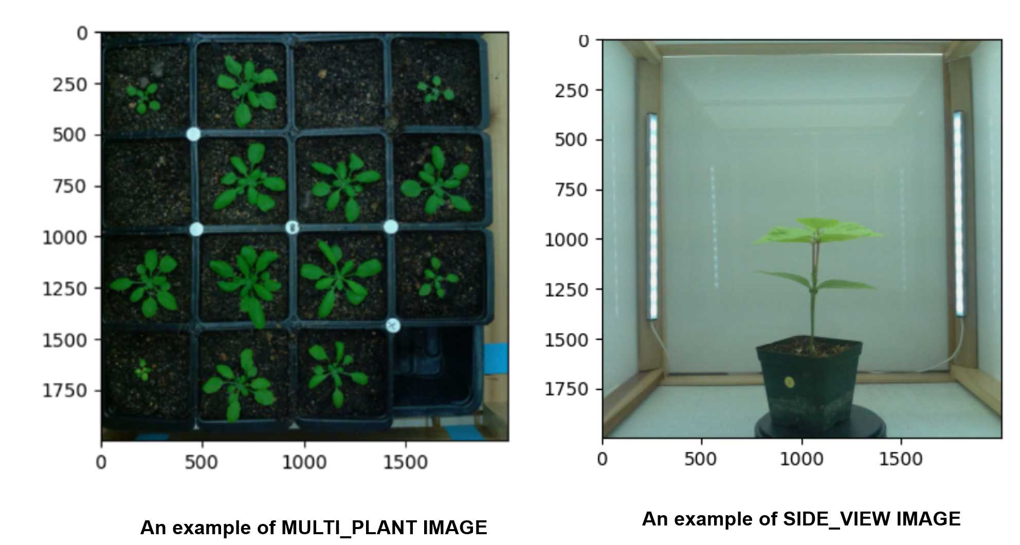
Parameter for MULTI_PLANT IMAGES
The pipeline for MULTI_PLANT IMAGES was based on the PlantCV tutorial https://plantcv.readthedocs.io/en/v3.2.0/multi-plant_tutorial/with some modifications and optimizations. Parameters associated with five parts, including:
1. position and white-balance corrections
2. image color space transformation
3. image masking
4. selection of regions of interest (ROIs)
5. extraction phenotypes from each individual plant
Each part will be tested to reach the optimum effects of phenotype data extraction. See tips for each part below:
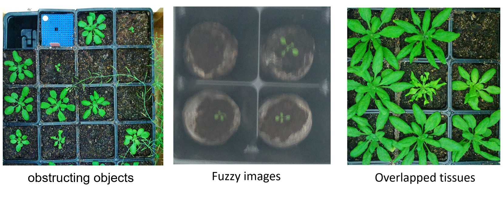
Before executing the pipeline for each part, a quick check of image quality will be necessary. For users' image data, the following bad examples should be excluded for parameter settings and analysis:
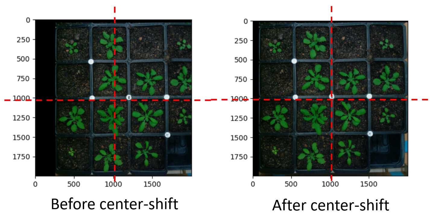
position and white-balance corrections
After the image loading, the initial step is shifting or rotating the image at the center by using shift functions. The step is necessary which provides a framework for the selection of regions of interest (ROI). Please see two examples below;
# Shift image. This step is important for clustering later on.
# For this image it also allows you to push the green raspberry pi camera
# out of the image. This step might not be necessary for all images.
# The resulting image is the same size as the original.

# Inputs:
#   img    = image object
#   number = integer, number of pixels to move image
#   side   = direction to move from "top", "bottom", "right","left"
imgs = pcv.shift_img(img=img1, number=80, side='left')
img1 = pcv.shift_img(img=imgs, number=20, side='top')
Followed by white-balance correction, color can be compared across images so that image processing can be the same between images
#Normalize the white color so you can later
# compare color between images.
position, y position, box width, box height)# white balance image based on white balance spot
img1 = pcv.white_balance(img, roi=(1400,900,100,100))
```<img src="https://static.yanyin.tech/literature_test/protocol_io_true/protocols.io.8epv59oz4g1b/jxb5bhvs77.jpg" alt="" loading="lazy" title=""/>
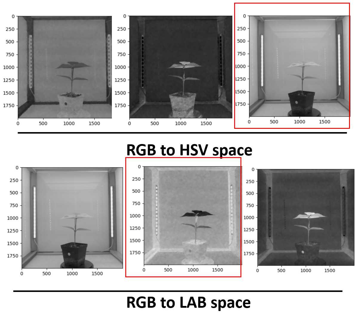
**image color space transformation**
The transformation from RGB to LAB color space is the preliminary step to isolating the plants from the background based on the nature of contrast between green objects and the background. In this protocol, we selected the "a" channel which brings the highest level of contrast between plant tissues and background.
**See code for color space transformation as below:**
l = pcv.rgb2gray_lab(rgb_img=img1, channel='l') a = pcv.rgb2gray_lab(rgb_img=img1, channel='a') b = pcv.rgb2gray_lab(rgb_img=img1, channel='b')
<img src="https://static.yanyin.tech/literature_test/protocol_io_true/protocols.io.8epv59oz4g1b/jxbrbhvs78.jpg" alt="" loading="lazy" title=""/>

 **image masking**


Effective masking from LAB transformed binary images requires the well-defined edge of plant tissues and background. Thus, a good cut-off for transformation should be selected. Attached is one example with over-masked, good-mask, and less-masked images being processed (from left to right).

<img src="https://static.yanyin.tech/literature_test/protocol_io_true/protocols.io.8epv59oz4g1b/jxcdbhvs79.jpg" alt="" loading="lazy" title=""/>

 **See the**   **code for masking below:**
Set a binary threshold on the saturation channel image
Inputs:
gray_img = img object, grayscale
threshold = threshold value (0-255)
max_value = value to apply above threshold (usually 255 = white)
object_type = light or dark
- If object is light then standard thresholding is done
- If object is dark then inverse thresholding is done
img_binary = pcv.threshold.binary(gray_img=a, threshold=110, max_value=255, object_type='dark')
 **selection of regions of interest (ROI)**


The ROIs define the individual plants to be included for extracting phenotypes. The coordinates of the X and Y-axis of the left-upper corner of the region, H and W are corresponded to the height and width of the ROI.
Define region of interest (ROI)
Inputs:
img = An RGB or grayscale image to plot the ROI on.
x = The x-coordinate of the upper left corner of the rectangle.
y = The y-coordinate of the upper left corner of the rectangle.
h = The width of the rectangle.
w = The height of the rectangle.
roi_contour, roi_hierarchy = pcv.roi.rectangle(img=img1, x=45, y=40, h=1900, w=1900)
<img src="https://static.yanyin.tech/literature_test/protocol_io_true/protocols.io.8epv59oz4g1b/jxbzbhvs73.jpg" alt="" loading="lazy" title=""/>

Based on ROIs selected, a detailed division of an individual plant will be defined using a circle with a fixed circle radius. To realize a better segmentation purpose, plants should be placed at the center of the coordinate circle.
img = The image with ROI defined
coord = The x-coordinate and y-coordinate of the upper left corner of the
radius = The radius of the blue circle over each individual plant
spacing = the height and width of the distance between two circles
nrow = the number of circles in the horizontal direction
ncols = the numbers of circles in the vertical direction
rois1, roi_hierarchy1 = pcv.roi.multi(img=img1, coord=(285,285), radius=160, spacing=(475, 475), nrows=4, ncols=4)
<img src="https://static.yanyin.tech/literature_test/protocol_io_true/protocols.io.8epv59oz4g1b/jxchbhvs74.jpg" alt="" loading="lazy" title=""/>

 **extraction phenotypes from each individual plant**


The final phenotype extraction will be performed based on small regions defined for each plant along with results being saved with a numeric ordering (from 0-15) and planting pots without plants will be skipped.


<img src="https://static.yanyin.tech/literature_test/protocol_io_true/protocols.io.8epv59oz4g1b/jxbmbhvs75.jpg" alt="" loading="lazy" title=""/>

The final output will be generated along with the edge of leaves being marked. Check if most of the desired leaf area was covered by blue edge lines.
Parameter for SIDE_VIEW IMAGES
The pipeline for SIDE_VIEW IMAGES was refered based on PlantCV tutorial https://plantcv.readthedocs.io/en/stable/tutorials/vis_tutorial/ with some modifications and optimizations. Parameters assiocaited wtih five parts, including:
1. position and white-balance corrections
2. image color space transformation
3. image masking
4. selection of regions of interests (ROIs)
5. extraction phenotypes from a plant
position and white-balance corrections
After the image loading, shifting or rotating image is optional. If adjustment of position is needed, refer code from the MULTI_PLANT IMAGE protocol for details. Also, white balance correction is optional as shown below:
# Corrects image based on color standard and stores output as corrected_img
corrected_img = pcv.white_balance(img=img, mode='hist', roi=[450, 1250, 100, 100])
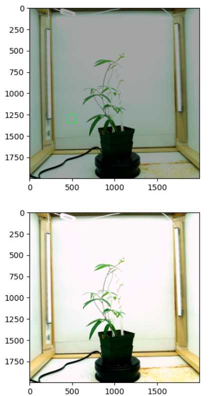
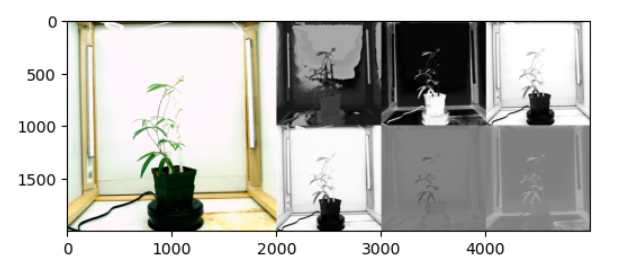
image color space transformation
Effective masking from LAB and HSV transfomred binary images requires the well-defined edge of plant tissues and background. Thus, a good cut-off for transformation should be selected. In side-view image pipeline, we applied slightly different strategy by combining two separate binary images into the same channel. Specicically, we selected the V and A channel for channel integration.
Initially, users can visulize all channels at a glance for transformation. With our setups, the A and V channels are recommended and we'll merge two channels as follow
# Examine all colorspaces at one glance
colorspace_img = pcv.visualize.colorspaces(rgb_img=corrected_img)
a_thresh = pcv.threshold.binary(gray_img=a, threshold=105, max_value=np.max(a), object_type='dark')
v_thresh = pcv.threshold.binary(gray_img=v, threshold=220, max_value=np.max(a),object_type='dark')

### combine v and a channel for the subsequent step
v_a = pcv.logical_or(bin_img1=v_thresh, bin_img2=a_thresh)

### apply the masking
masked = pcv.apply_mask(img=img, mask=v_a, mask_color="white")
``` **selection of regions of interests (ROIs)**
mnasked = An grayscale image to plot the ROI on.
x = The x-coordinate of the upper left corner of the rectangle.
y = The y-coordinate of the upper left corner of the rectangle.
h = The width of the rectangle.
w = The height of the rectangle.
roi1, roi_hierarchy = pcv.roi.rectangle(img= masked, x=450, y=400 , h=1000 , w=1120)
roi_objects, hierarchy3, kept_mask, obj_area = pcv.roi_objects(img = img, roi_contour=roi1, roi_hierarchy=roi_hierarchy,object_contour=id_objects,obj_hierarchy= obj_hierarchy, roi_type="partial")
 **extraction phenotypes from a plant**


For side view images, taking images from seven angles will be recommended as representatieve input to describe leaf area of the entire plants. Quality control from image each angle per plant will be necessary before proceeding to the next batch analysis step. See examples which represent the good quality image as below:
extract leaf area based on masked images
analysis_image = pcv.analyze_object(img=img, obj=obj, mask=mask)
<img src="https://static.yanyin.tech/literature_test/protocol_io_true/protocols.io.8epv59oz4g1b/jxcvbhvs712.jpg" alt="" loading="lazy" title=""/>
