Trinity College Botanic Garden long-term monitoring program
Midori Yajima, Michelle Murray, Jennifer McElwain, Stephen Waldren
Long-term
monitoring
plant
ecology
stomatal conductance
pollution
PM10
PM2.5
trees
climate change
botanic garden
physiology
chlorophyll
water use efficeincy
fluorometry
Disclaimer
Abstract
Botanic gardens hold large, documented, and accessible collections of living plants. These represent unique subsets of taxa from different biogeographical regions growing under common environmental conditions, connecting people to global plant research and conservation efforts while offering a place beneficial for human health and wellbeing. Despite Botanic Gardens being an ideal setting for climate change research, their potential for comparative, long-term studies and outreach in the field is still underutilised. As part of its ten year strategy, Trinity College Botanic Garden (TCBG) aims to tap this potential and establish a programme for long-term (>30 years) monitoring of key physiological performances in its living woody plant collection. The programme will also assess particulate pollution (PM10 and PM2.5) interception by the same trees, pairing climate change and urban green research. Importantly, the project will include the design of a transferable protocol, produce vouchered herbarium specimens as a future historical archive and as a pedagogical tool, and support the garden outreach strategy, so as to nurture its link with both Trinity College Dublin and local communities, ensuring the garden’s legacy into the future.
Before start
Steps
Plant physiology
When June, not later than mid-July (end of the growing season).Make sure plants are not water stressed, e.g. do not perform measurements after prolonged dry spells.
Leaf selection
1.1.1 Select 3 leaves/ leaflets/ phyllodes (from here on all referred to as leaves) per tree
1.1.2 Per each leaf
- Tag leaf with a ribbon 1 1 reporting a code that will work as leaf ID (e.g. the first leaf measured on Arbutus unedo will be AU01)
- Make note of leaf orientation (the N/S/E/W direction the leaf is facing)
- Make note of GPS 2 2 position of the tree (for any tree that have not been measured in previous years)
Porometry
Using porometer3, to measure plants' stomatal conductance (gs) 3, to measure plants' stomatal conductance (gs)
1.2.1 1.2.1 Take 1 porometry reading x each leaf x each tree
- Once per day between 08:30 h and 14:00h
- Over 3-5 consecutive days. To account for the natural day-to-day variability in gs for each species under ambient conditions, follow a different order of trees and leaves measured every day.
Note
Equipment-related:Calibrate every day or if temp changes of ca 15 °CMeasure at the prevailing microclimate condition of that dayMeasure in automatic mode - measures continuously and derive best estimate for leafLeaves-related:Measure at the interveinal areolae at mid-lamina of the abaxial surface. In the case of compound leaves, measure the terminal leaflet; for larger leaves clamp the sensor as far onto the leaf as possible, taking care to avoid damage to the leaf marginMeasure leaves at the same position in the crown (e.g. base level, arm reach), to normalise for gs changes with tree heightMeasure always at the same position (e.g. right blade of leaf that face me)During the measuremets:Minimise factors interfering with the readings (look away or wear mask to avoid changing CO2 conditions locally, move the leaf as little as possible)Name readings with each leaf ID
1.2.2 Download data 1.2.2 Download data from the porometer at the end of each day
- Download software from website (see Resources below)
- Follow instructions as reported in the porometer's manual 1.2.3 Store data in double copy (e.g. computer/ hard drive and Google Drive)
Chlorophyll content and environmental data
Using PhotosynQ 4 , to measure chlorophyll content and environmental variables at the leaf level (PAR, temperature etc.)
1.3.1 1.3.1 Download the mobile app (needs and Android phone), set a project to record observations
1.3.2 1.3.2 On the same tagged leaves used for porometry (possibly clamping the same portion), soon after or right before porometry, take 1 reading x each leaf x each tree. Annotate leaf ID on the app after every measurement.
1.3.3 1.3.3 Data will be uploaded automatically to the project online, but make sure to download them from the website at the end of every day.
1.3.4 Store data in double copy (e.g. computer/ hard drive and Google Drive)
Fluorometry
Using Pocket pea5, to measure chlorophyll fluorescence 5, to measure chlorophyll fluorescence
1.4.1 At the end of the day 1.4.1 At the end of the day, clip 1 leaf x 15 leaves x tree.
- There won't be enough leaf clips for measuring all the trees, so it will be necessary to repeat this every day until all the trees will be assessed. This will have to be done only once per tree and not repeated over the 3-5 days, as chlorophyll fluorescence won't change much over that period
1.4.2 Close each slide on leaf clips to dark adapt leaves, and leave for the night
1.4.3 Take measurements as the first thing in the following morning
-
Place pocket pea on each clip covering the opening, slide clip open, take measurement, take clip off 1.4.4 Download data
-
Download PEA+ Software from website
-
Connect Pocket pea to software through USB port
-
Download all data
-
Erase data from instrument 1.4.5 Store data 1.4.5 Store data in double copy (e.g. computer/ hard drive and Google Drive)
Water use efficiency (WUE)
Obtained by analysing 13C Obtained by analysing 13C isotopes ratio from leaves samples
1.5.1 1.5.1 On the last day of fieldwork, take the same tagged leaves used for porometry and sort them in separate envelopes6, pencil the leaf ID on the envelopes
1.5.2 1.5.2 Oven dry at 50-60 °C for 2 days in TCD plant atmosphere lab
1.5.3 In the plant atmosphere lab, for each sample take a fragment of the dried leaf and grind it with mortar and pestle 7 7 into a fine powder
1.5.4 Sieve 10 10 powder on an aluminium 11 11 foil
1.5.5 Transfer powder into an eppendorf 12 12 and label with leaf ID
1.5.6 In the anatomy lab, transfer ca. 3 mg of powder into tin foil capsules 13 13 using a spatula14and fold them using two tweezers 15 15 into small quadrats of <5 mm length
1.5.7 Sort samples in a 96 well tray16, keeping track of the position of each sample and correspondent leaf ID
1.5.8 Place an order to the Stable Isotope Facility (SIF) in UC Davis for 13C analysis, pack the tray following the guidelines on their website (stating Prof. Jennifer McElwain as PI of the lab) and send it. Turnaround times are expected to be of ca. 2-3 months.
1.5.9 Once data come back, derive WUE from the isotope ratio using formula from Soh et al.2019
1.5.10 Store data in double copy (e.g. computer/ hard drive and Google Drive)
Weather data
Take weather data from the garden MET station
- Download/ obtain Campbell scientific LoggerNet software
- Download readings from the 30 days before the monitoring (monitoring days included) from the weather station, using a USB to RS232 cable
Data management
- Clean data (variable names in lowercase and no spaces, keep only relevant info), for porometry, PhotosynQ, WUE, fluorometry, and MET dataset. See the script "R/Monitoring_data.R" in the GitHub repo as a reference (link in Resources below). To push changes, please branch the main repo before, and once all changes are made create a pull request to merge it back.
- Convert final dataset in .csv format , as the preferred format for reproducibility (not necessary if the script "R/Monitoring_data.R" is followed as all datasets are automatically saved in that format).
Particulate Matter analysis
When Collection must be after a period of 5 to 10 days of dry weather and low wind, to avoid particulates to be washed away from the leaves. It has to be close in time to the plant physiology fieldwork.
Leaf selection
- 3 leaves x tree , choosing leaves close to the ones used for the physiological assessment (same branch, similar dimension and orientation if possible)
Leaf collection and dehydration
2.2.1 2.2.1 Pick leaves and tag them with a leaf ID (can be the same used for the leaves nearby used for the physiology work) + progressive numbering. The latter will be the stub ID that will be used in Scanning Electron Microscopy (SEM) later
2.2.2 2.2.2 Wrap leaves in lint-free tissue 17 17 to avoid contamination from paper fibres or other sources while pressing
2.2.3 2.2.3 Dehydrate leaves in plant press18 18 for approx. 2 weeks, changing newspapers 19 19 regularly. Leaves need to be pressed and not oven dried so that can be imaged correctly under the SEM later
2.2.4 2.2.4 Sort dried leaves in separate envelopes 6 6 reporting leaf ID and sample ID, keeping them wrapped in lint free tissue
Samples preparation in the Centre for Microscopy and Analysis lab
2.3.1 2.3.1 Cut 1 sample of 0.5 x 0.5 cm ca from each leaf with single edged blade20
2.3.2 Prepare SEM stubs21 with conductive tabs22
2.3.3 Using tweezers 15, 15, mount 1 sample x stub and press firmly with lint-free tissue
2.3.4 Paint the edges of the sample with carbon paint24 (pure graphene) to prevent curling while in the SEM
2.3.5 Mark the bottom of the stub with the unique stub ID that was given during collection
2.3.6 Leave samples mounted on the stubs to dry out for 1-2 days
Initialise TESCAN MIRA3 TIGER SEM
2.4.1 Initialise SEM by hitting STANDBY button on screen to get it out of standby mode
2.4.2 2.4.2 Hit VENT button to vent the chamber and be able to open it
2.4.3 When the carousel in the stage control panel (bottom left screen) becomes red, click on central sample in carousel to make it advance
2.4.4 Open chamber, pull carousel out making sure it doesn't hit the central lens, and insert the stubs in the carousel noting down the stub ID per each position in the carousel. Screw stubs in carousel lightly, then put carousel back in and close chamber
2.4.5 Hit PUMP button to pump chamber again
2.4.6 Type 0 in stage control panel (bottom left screen) at the position X to move stage back into place. Hover mouse over stop button to interrupt movement, just in case
2.4.7 Type 15 mm in stage control panel (bottom left screen) at the position WD & Z to move stage at the right distance. Hover mouse over stop button to interrupt movement, just in case
2.4.8 Hit BEAM ON to turn the beam on, scroll mouse wheel to control screen “updating” speed
2.4.9 Right click on image on bottom left screen and select "auto bright contrast" to adjust the contrast of the image 2.4.10 0 Find an object to visualize and and hit Adjustment option in bottom right screen, then align instrument from the top down hitting Auto gun, Auto column centring, Manual column centring. The last one will open a window, where to click on WOB, increase magnification if necessary by scrolling the wheel on the console, and adjust the ball on the console by moving it left/ right until image is not moving anymore
2.4.11 Hit Magnet button on bottom right screen to degauss. This will prevent magnetism in the chamber that could affect image quality and measurements
2.4.12 Set microscope settings, On the Aztec software (top right screen), make a new project and switch on EDS Sensors from Aztec interface (bottom right icons) > Position > In
Map elements at SEM
2.5.1 Turn IR light off right-clicking on bottom right image
2.5.2 Selecting SE in the Channel A entry from SEM detectors & Mixer panel if any area is charging, and analyse only areas that are not
2.5.3 Put back BSE option in Channel A entry
2.5.4 For each sample, pick 3 random areas, increase magnification up to 800 X
2.5.5 Map section in Aztec, make new site for every area analysed in the "data tree" window, and label it meaningfully e.g. 1st area analysed of leaf CS01 will be CS01_01
2.5.6 In Scan image section, hit Play button to scan the image 2.5.7 7 In Acquire map data, hit Play button to map elements
2.5.8 Turn SEM off once finished by going at low magnification, hitt In Acquire map data, hit Play button to map elements
Feature analysis
2.6.1 Download project from SEM on hard drive
2.6.1 Upload project on offline computer and start it
2.6.2 Go on feature analysis option
2.6.3 On the Detect feature tab, right click on image (only electron image, not the composite), export as tiff, name with subsample ID
2.6.4 2.6.4 Threshold features by appearance on Detection refinement window.
Adjust the selection window to select relevant part of the spectrum corresponding to particles by appearance (PM will be distinguishable from the background, can be selected highlighting lighter part of the spectrum for heavy metals, darker for carbon-based particulates).
Adjust filter settings to better select PM (e.g. use erosion filer if feature is bigger than actual PM when observed in the background). Features should be detected automatically, if not hit detect features
2.6.5 On acquire site window
On Data tab, check morphology, chemistry, area, field, class boxes
Extract to get chemical data. Make sure to click on the whole site (not on electron image) or it will not get data
Select artefacts (features that were selected by mistake) from the image using the option “Select feature at the point of the image”, and remove it using “Reject function bottom of the Data/ Summary/Single section
2.6.6 On acquire site window file as the subsample and delete summary rows at the bottom (mean, etc.). Repeat for all the subsamples.
Data management
- Merge datasets and clean data (variable names in lowercase and no spaces, keep only relevant info). See the script "R/Monitoring_data.R" in the GitHub repo as a reference (link in Resources below). To push changes, please branch the main repo before, and once all changes are made create a pull request to merge it back to the main branch.
- Convert final dataset in .csv format , as the preferred format for reproducibility (not necessary if the script "R/Monitoring_data.R" is followed as all datasets are automatically saved in that format).
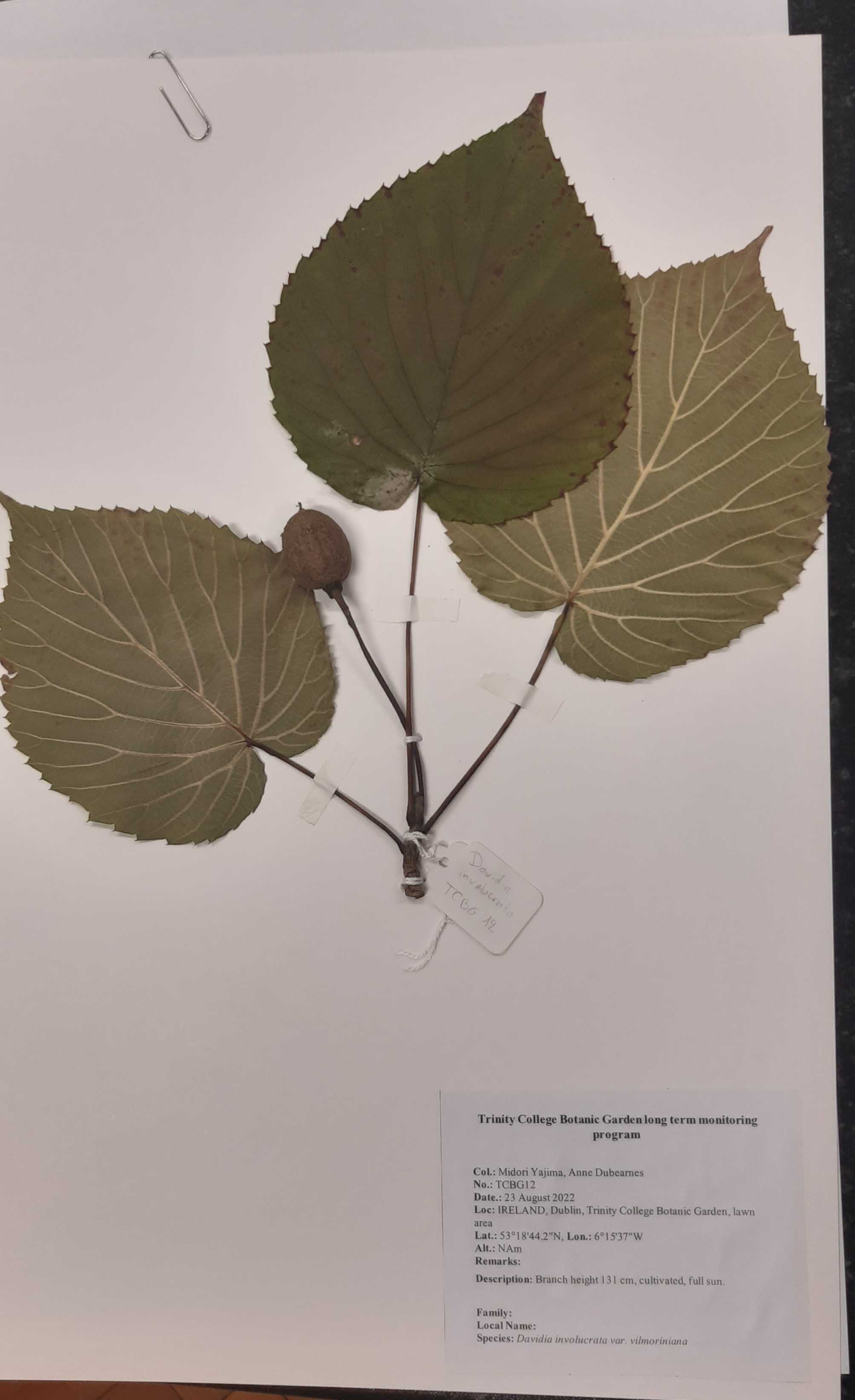
Herbarium sheets
When Collection must happen soon after the last day of plant physiology fieldwork. It must be in dry weather to avoid specimens rotting or developing moulds.
Selection of the specimen
3.1.1 Select and pick 1 specimen x tree for the actual herbarium sheet + 2/3 extra leaves (or leaflets) to preserve for any future analysis. Tag specimens with leaves tags26 26 reporting species (to avoid mislabelling later)
3.1.2 3.1.2 Label each specimen annotating species name
3.1.3 3.1.3 Separately, make note of
- Species name
- Specimen ID , as "TCBG sample-number" e.g. "TBCG1". Each specimen ID must be unique, so latest specimens have to continue the numbering of the herbarium sheets made in previous years. See resources in Section 3.3 for a link to labels of specimens of previous years
- Date
- Collectors
- Coordinates (can be taken from previous specimens)
- Location in the garden (e.g. walled garden, west arboretum etc. can be taken from previous specimens)
- Notes , including branch height when on the tree, ecological notes
3.1.4 3.1.4 Place specimen in plastic bag for transport (ideally one bag per specimen)
Preparation of specimens
3.2.1 3.2.1 Dehydrate plants in plant press18 within 12 hours from collection. Store the plant press in a dry place for approx. 2 weeks, changing newspapers regularly
3.2.2 3.2.2 Once ready, drop the press with all the specimen in the Herbarium freezer inside the Botany Department for at least 72 hours, to kill any residual mold.
Creating herbarium labels
3.3.1 3.3.1 See the script "R/ Herbarium label" in the GitHub repo as a reference (link in Resources below). To push changes, please branch the main repo before, and once all changes are made create a pull request to merge it back. Add own spreadsheet following the structure of files published in its "Data/ Herbarium data" section. Fill it with information noted in Section 3.1.3.
3.3.2 Manually move the generated .rtf file from the main repo to the dedicated folder in "Outputs/Herbarium labels"
Mounting of herbarium specimens
3.4.1 Mount specimens on herbarium sheets, making sure to
- Stitch specimens instead of using glue. Use glue only if necessary (e.g. specimen is too heavy, there are too many leaves) so that each specimen can be removed and used for future analyses
- Storing the extra leaves in a separate paper bag attached to the sheet
- Printing and attaching herbarium labels reporting the information noted on the field
3.4.2 3.4.2 Lay herbarium sheets away in Trinity Herbarium
- Check for Herbarium ID numbers for the species in the Herbarium book
- Seek out the respective cabinet with the ID number
- Lay in folders for the respective species, section "Cultivated"
Online data publishing
When
Once all data and metadata have been obtained and cleaned
Upload datasets to Dryad
4.1.1 Prepare a README file (see details in Resources below)
4.1.2 Follow steps reported in Dryad's website to create new version of dataset (see details in Resources below) . This requires login details of first author, please reach out at yajimamidorimichela@gmail.com
Data visualization for the Witness Tree Project webpage
When
Once all data and metadata have been obtained and cleaned
Create visualization
5.1.1 See the script "R/Viz for website" in the GitHub repo as a reference (link in Resources below). To push changes, please branch the main repo before, and once all changes are made create a pull request to merge it back. Please note that the script needs cleaning, for any issue reach out to Midori Yajima (yajimamidorimichela@gmail.com)
5.1.2 Send materials to designated garden staff to be uploaded in Trinity College Botanic Garden's website
Updating monitoring records
When
At the end of field/ lab work
Update records for the monitoring
6.1.1 6.1.1 Branch the GitHub repo (link in Resources below) and update the file in "Data/Tree_list". In particular, update the "Monitoring record" tab with details on year, month, features monitored, staff involved.
6.1.2 Create a pull request to merge changes made to the main repo
Update protocol (optional)
If any changes were implemented during the field or lab work, update this protocol either by creating a fork or versioning the original one. The latter will require login details from one of the authors (reach out to yajimamidorimichela@gmail.com)
