Past human stone tool performance: experiments to test the influence of raw material variability and edge angle design on tool function

The research question behind this here presented experiment is based on archaeological artefacts, so-called Keilmesser from the Late Middle Palaeoltihic. The artefacts are from the sites of Balver Höhle, the Upper site of Buhlen (both Germany) and Grotte de Ramioul (Belgium). For more information about the sites see the following (exemplary) references:

3D scanning

In total 175N Keilmesser were analysed and scanned with an AICON smartScan-HE R8 from the manufacturer Hexagon (software version OptoCat 2018R1). The S-150 FOV (field of view) used has a point-to-point distance of 33 µm.

Equipment

Value	Label
smartScan-HE R8	NAME
3D structured light scanner	TYPE
AICON	BRAND
-	SKU
S-150 FOV, resolution of 33 µm	SPECIFICATIONS

Software

Value	Label
OptoCat	NAME
Hexagon Manufacturing Intelligence Software	DEVELOPER
2018R1	VERSION

The scanning settings are identical to the following protocol, and details can be found there:

Enhancing lithic analysis: Introducing 3D-EdgeAngle as a semi-automated 3D digital method to systematically quantify stone tool edge angle and design

The editing steps to create a closed 3D model are also the same as in the protocol mentioned above and were executed with GOM inspect, a free software for 3D measurement data.

Software

Value	Label
GOM Inspect	NAME
Hotfix 2, Rev. 111729, build 2018-08-22	OS_NAME
GOM	DEVELOPER
https://www.gom.com/de-de/produkte/gom-inspect-suite	LINK
2018	VERSION

Edge angle calculation

The edge angle measurements on the 3D models of the Keilmesser were taken with 3D-EdgeAngle . For details about the method see (publication of the forthcoming paper):

Enhancing lithic analysis: Introducing 3D-EdgeAngle as a semi-automated 3D digital method to systematically quantify stone tool edge angle and design

For calculating the edge angles, the following parameters were applied:

• "2-lines" measuring procedure
• the length of the line was defined with 2 mm
• 10 mm as distance to the intersection
• only sections two to eight were used

Mean values were calculated in R, a free software and programming language for statistical computing and graphics.

Software

Value	Label
R Studio Desktop	NAME
The R Studio, Inc.	DEVELOPER
https://www.rstudio.com/products/RStudio/	LINK
1.1.463	VERSION

See "analysis_EA_Keilmesser" within the following repository on GitHub:

https://github.com/lschunk/PastHuman_StoneToolPerformance.git

Or in open access on Zenodo:

https://doi.org/10.5281/zenodo.7564605

Standardised tools

24 experimental standard samples were produced for the experiment:

6 x 35°

6 x 35°

6 x 45°

6 x 45°

Raw material

Baltic flint:

Southern Sweden (secondary deposit):

55.945852 N, 12.767851 E

Silicified schist:

Balver Höhle

51.339167 N, 7.871944 E

Buhlen

51.191022 N, 9.086585 E

Blanks

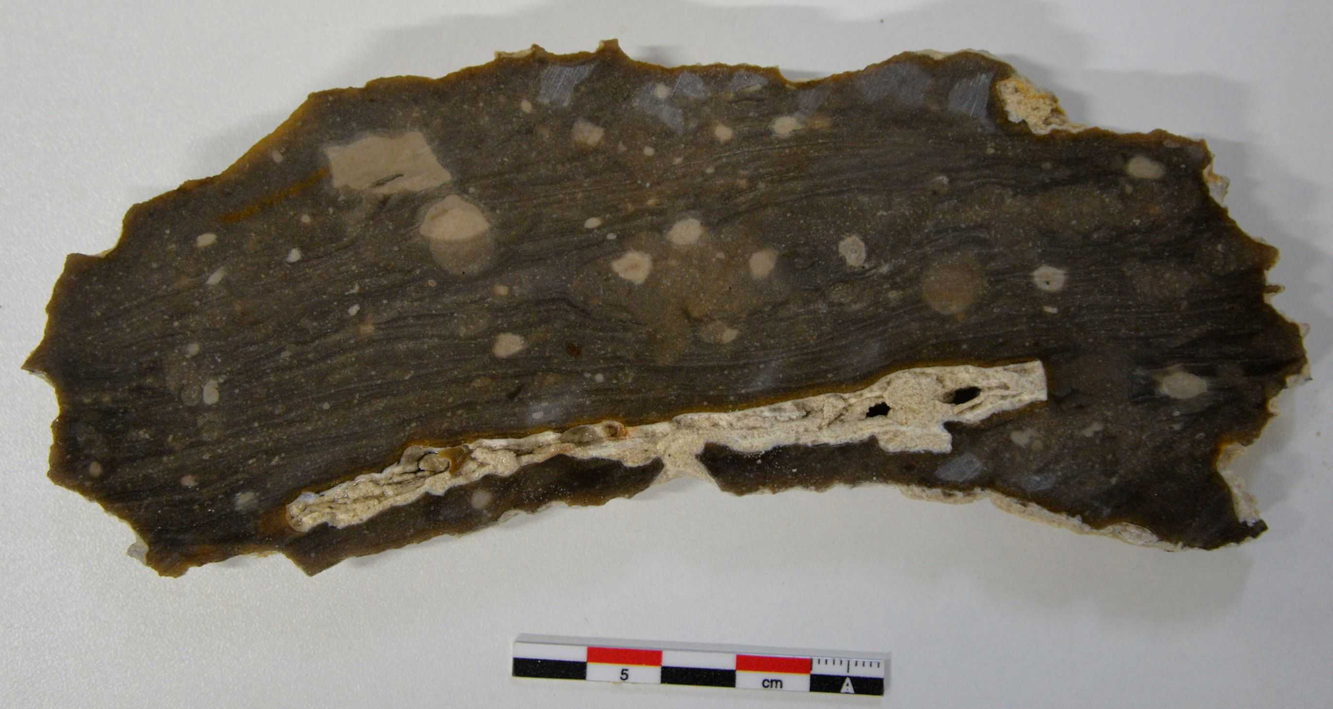
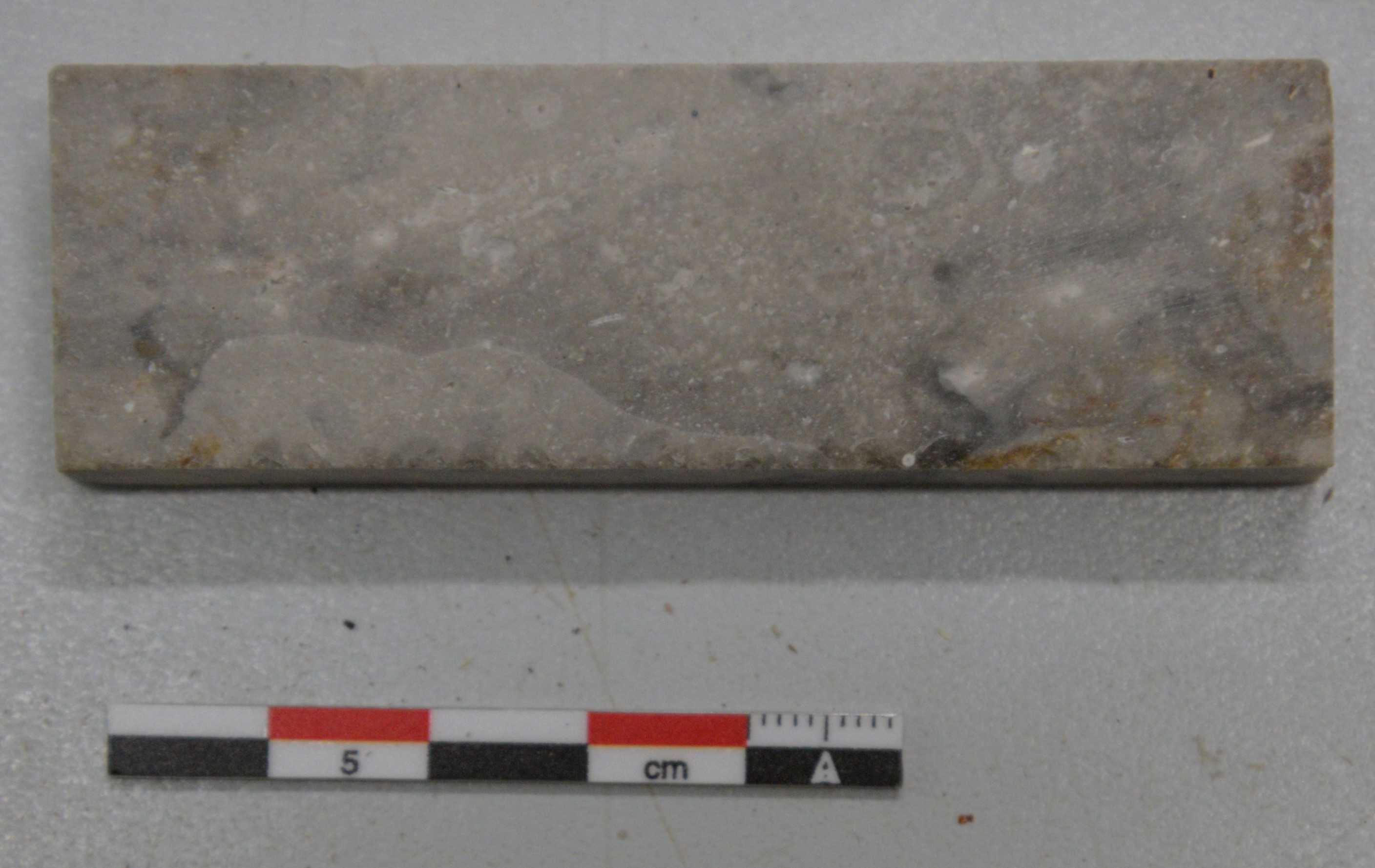
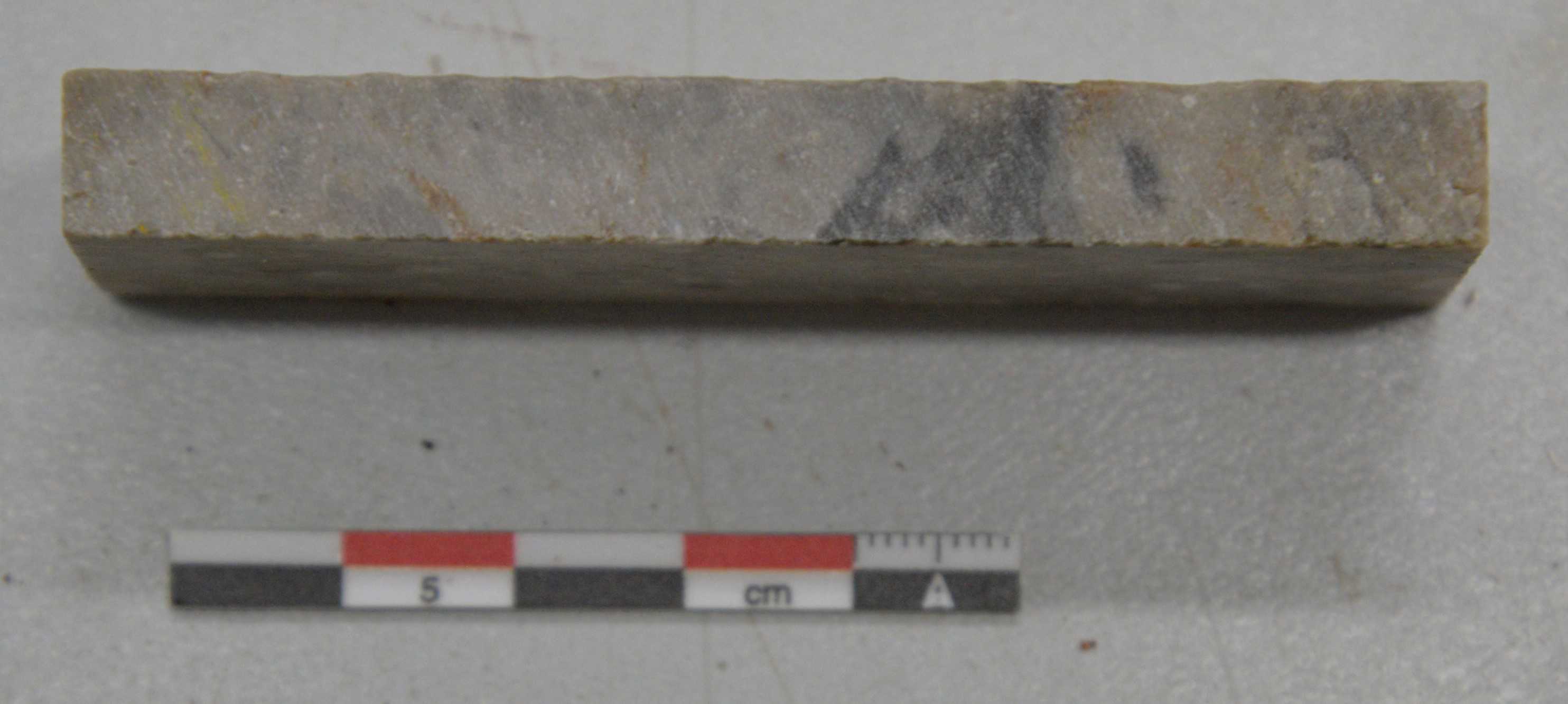
Raw material nodules/ blocks (step #2.1) were first cut into rectangular cuboids (blanks) of the following dimensions:

10mm

25mm

60mm

Equipment

Value	Label
Goliath 450	NAME
Lapidary rock saw	TYPE
Steinschleifmaschinen & Lapidary tools Ltd.	BRAND
-	SKU
-	SPECIFICATIONS

a) cut 10mm slices

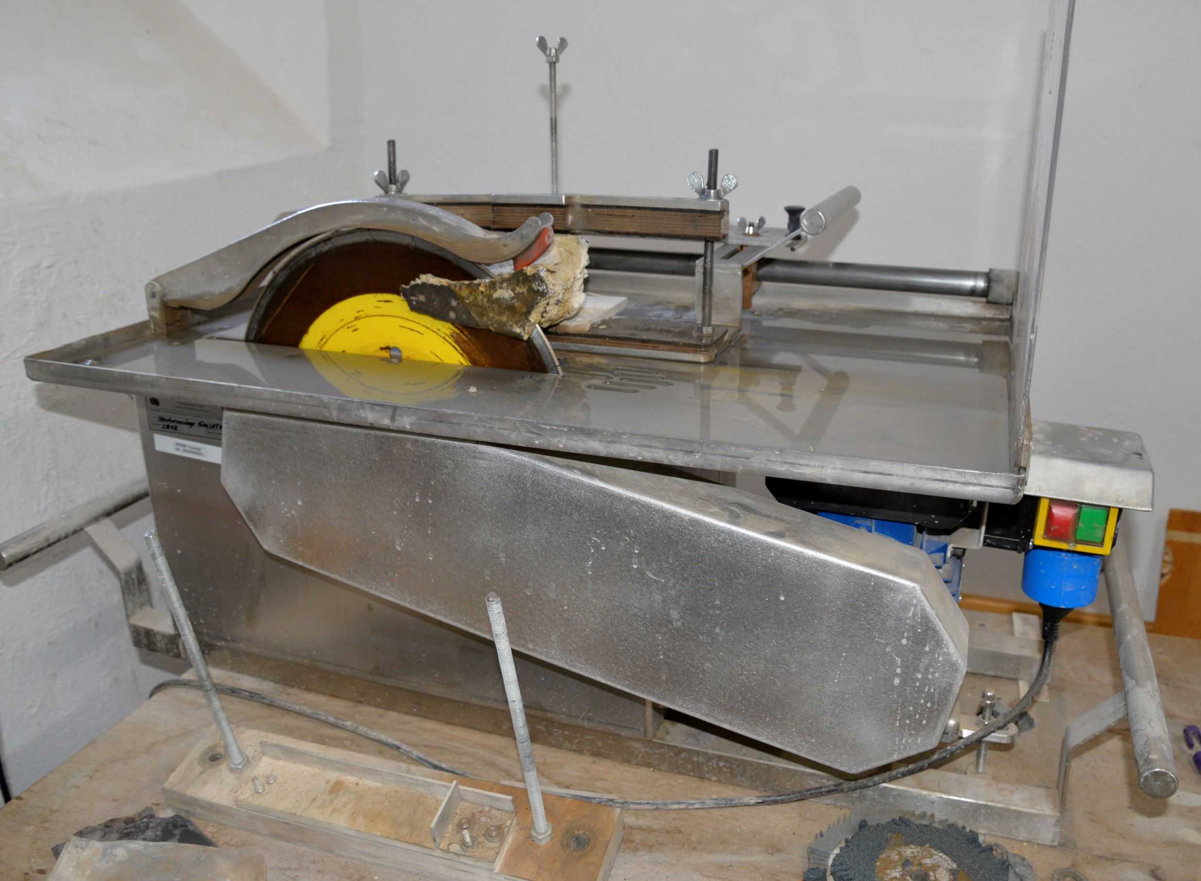
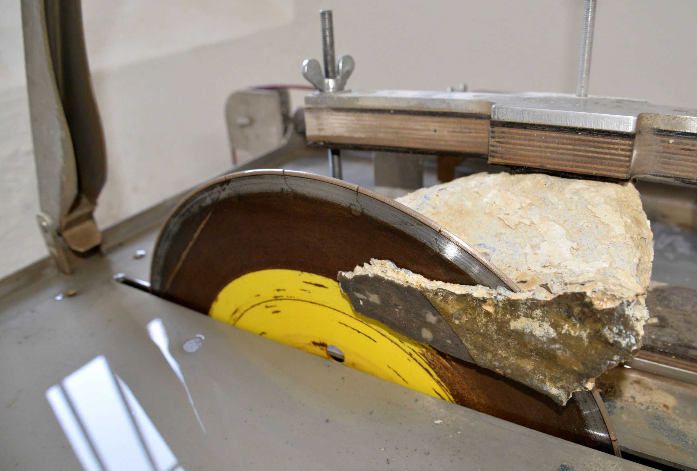
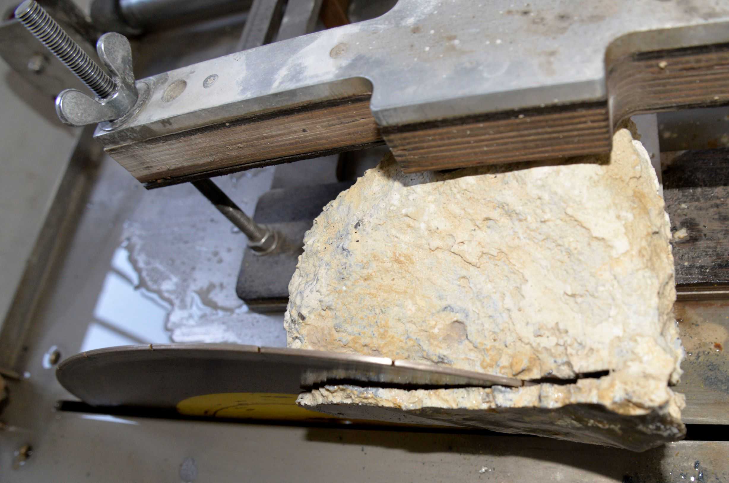
b) cut slices into blanks

Hardness measurement

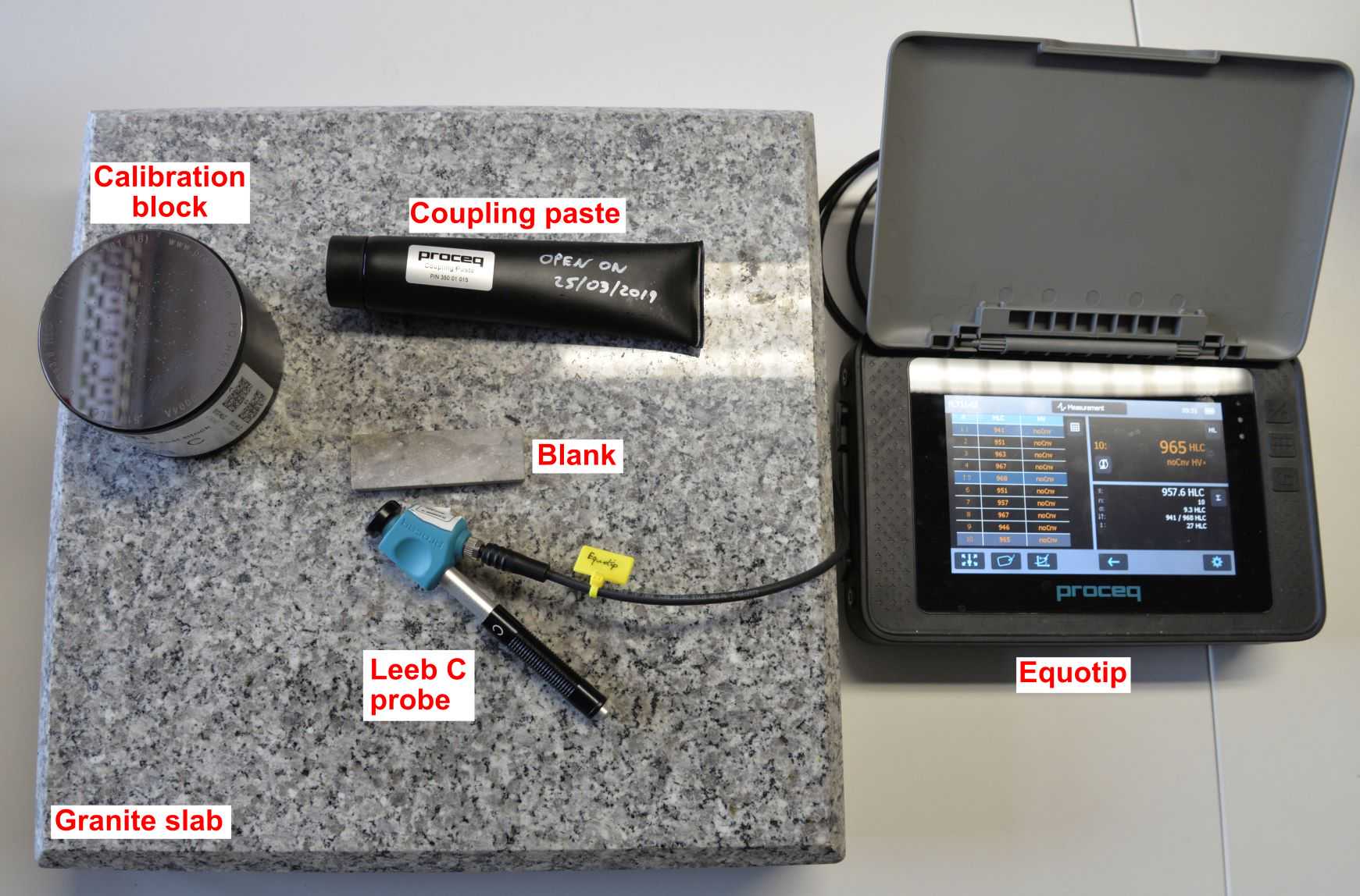
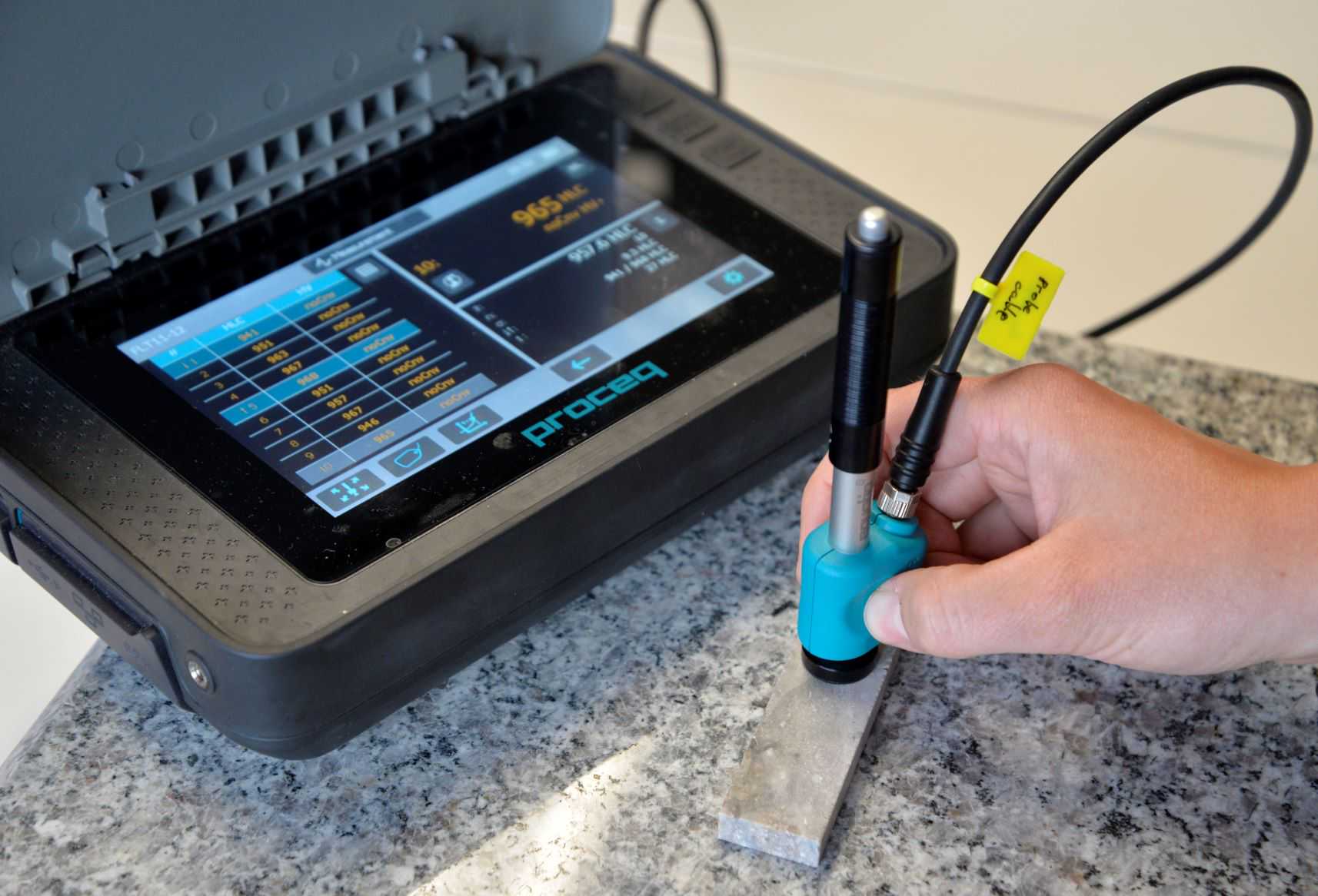
The hardness of the blanks (step #2.2) was measured with a Leeb rebound hardness tester.

Equipment

Value	Label
Equotip 550	NAME
Portable hardness tester	TYPE
Proceq	BRAND
-	SKU
Leeb C probe	SPECIFICATIONS

The blanks were placed on a stable base of sufficient mass (here a polished granite slab of about 20kg). Since the samples did not fulfill the requirements for minimum sample size and weight, coupling paste was used between the sample and the base. Each blank was measured ten times to insure and test intra-blank variability.

Edge angle

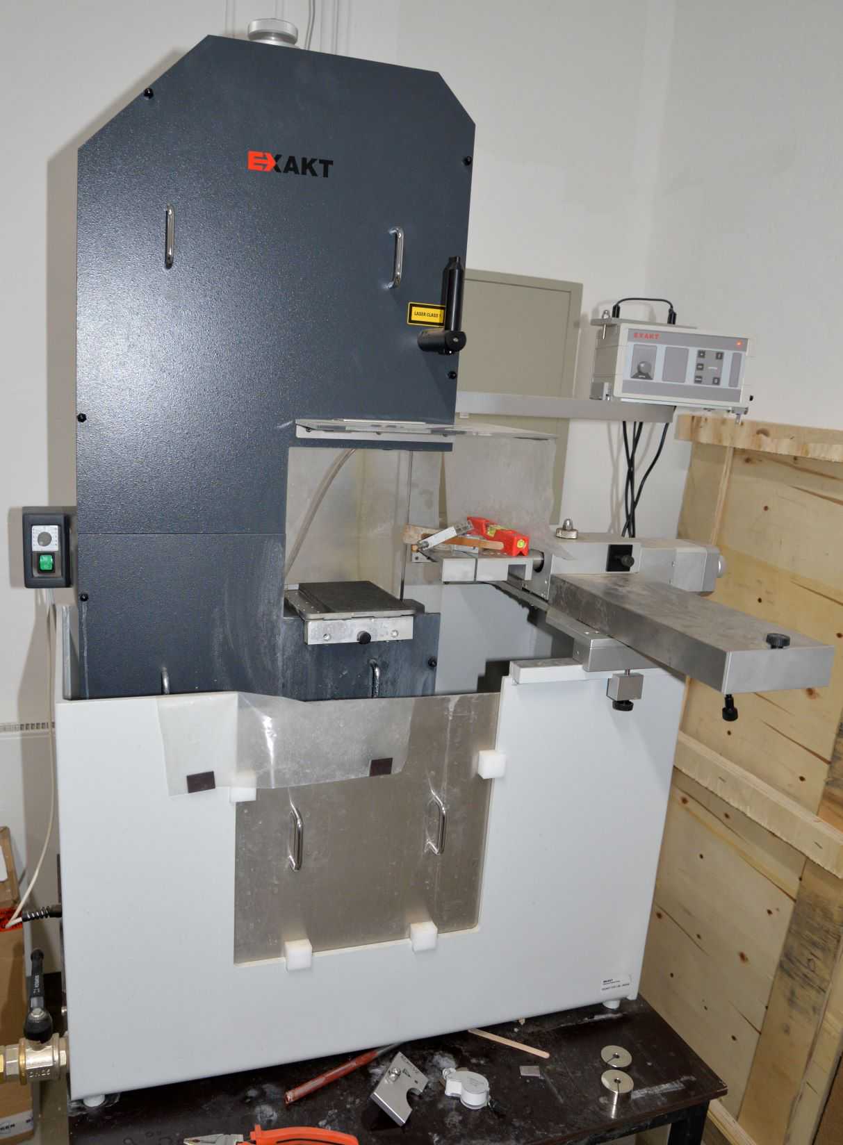
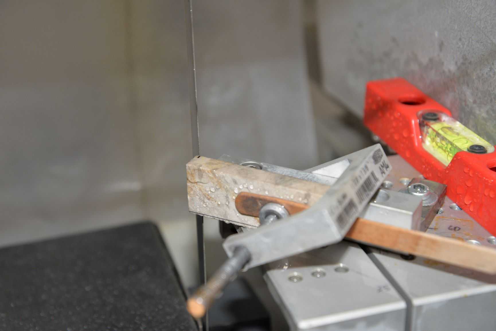
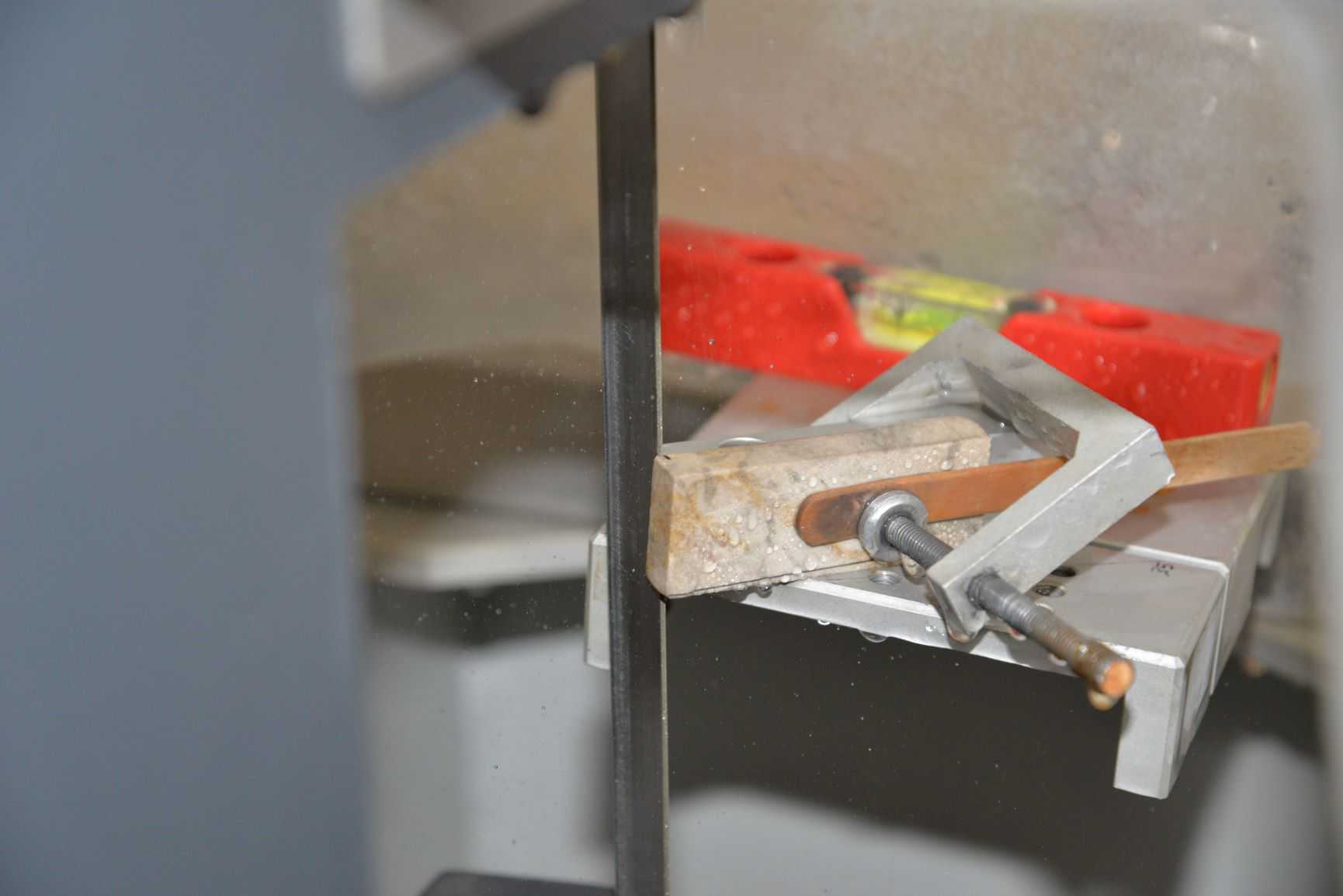
One end of the blanks (step #2.2) was cut to produce samples with a 35° / 45° , with the following dimensions:

10mm

25mm

30mm

Equipment

Value	Label
310 CP	NAME
Diamond band saw	TYPE
Exact	BRAND
-	SKU

<img src="https://static.yanyin.tech/literature_test/protocol_io_true/protocols.io.3byl4kr6ovo5/duehbgyf7.jpg" alt="Experimental standard sample without chamfered edge, view of side A (corresponding to the "dorsal" side of bifacial lithic artefact; here: flint)." loading="lazy" title="Experimental standard sample without chamfered edge, view of side A (corresponding to the "dorsal" side of bifacial lithic artefact; here: flint)."/>

<img src="https://static.yanyin.tech/literature_test/protocol_io_true/protocols.io.3byl4kr6ovo5/duejbgyf7.jpg" alt="Experimental standard sample without chamfered edge, view of side D (corresponding to the "lateral" side of bifacial lithic artefact; here: flint)." loading="lazy" title="Experimental standard sample without chamfered edge, view of side D (corresponding to the "lateral" side of bifacial lithic artefact; here: flint)."/>

Chamfered edge

To avoid catastrophic breakage of the edge during experiments, the leading edge of the experimental standard samples (step #2.4) was chamfered to a 45° (see #2.6 for photos).

Equipment

Value	Label
310 CP	NAME
Diamond band saw	TYPE
Exact	BRAND
-	SKU

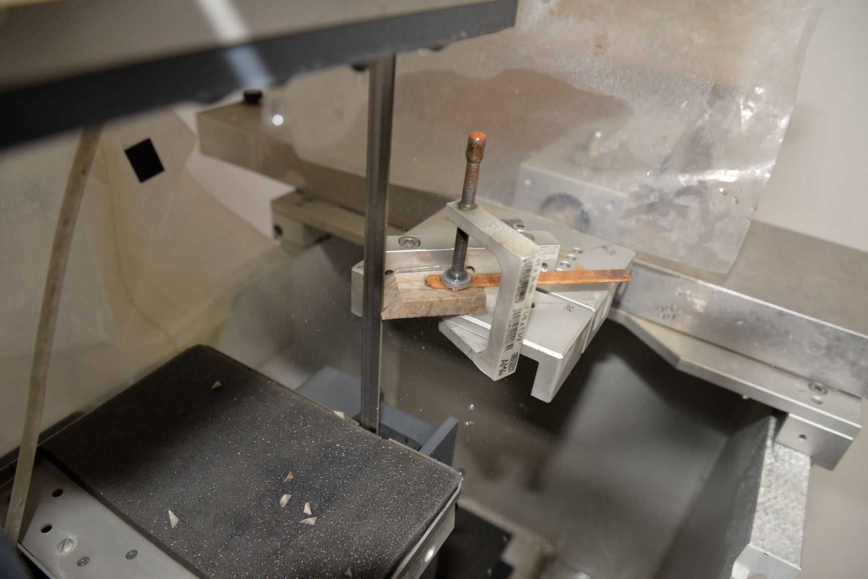
The cut with the band saw left a small burr between the two adjacent surfaces at the edge of the chamfered surface and the lateral side D. This burr was manually removed with a diamond drill bit in a mini drill.

Coordinate system

Three ceramic beads were adhered onto each side of the cutting edge to provide a coordinate system on each side.

<img src="https://static.yanyin.tech/literature_test/protocol_io_true/protocols.io.3byl4kr6ovo5/dyfcbgyf7.jpg" alt="Final experimental standard sample with beads, view of side A (corresponding to the "dorsal" side of bifacial lithic artefact; here: flint)." loading="lazy" title="Final experimental standard sample with beads, view of side A (corresponding to the "dorsal" side of bifacial lithic artefact; here: flint)."/>

<img src="https://static.yanyin.tech/literature_test/protocol_io_true/protocols.io.3byl4kr6ovo5/dye4bgyf7.jpg" alt="Final experimental standard sample with beads, view of side C (corresponding to the "ventral" side of bifacial lithic artefact; here: flint)." loading="lazy" title="Final experimental standard sample with beads, view of side C (corresponding to the "ventral" side of bifacial lithic artefact; here: flint)."/>

For details, see:

Summary of the standard sample production

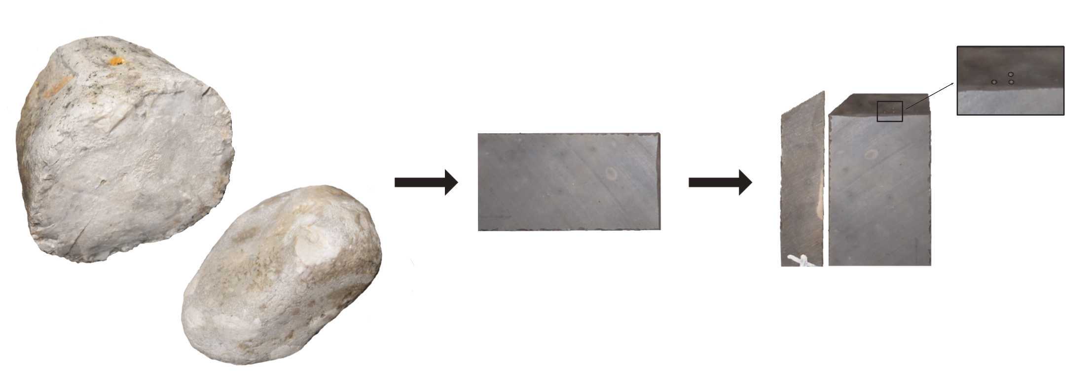
Cleaning

100mL

1Mass / % volume

Equipment

Value	Label
Sonorex Digitec DT255H	NAME
Heated ultrasonic bath	TYPE
Bandelin	BRAND
-	SKU
4.5 L	SPECIFICATIONS

40°C

0h 5m 0s

Standardised contact material

Three synthetic bone plates with the following dimensions were used as contact material:

250mm

250mm

6mm

75%

General settings

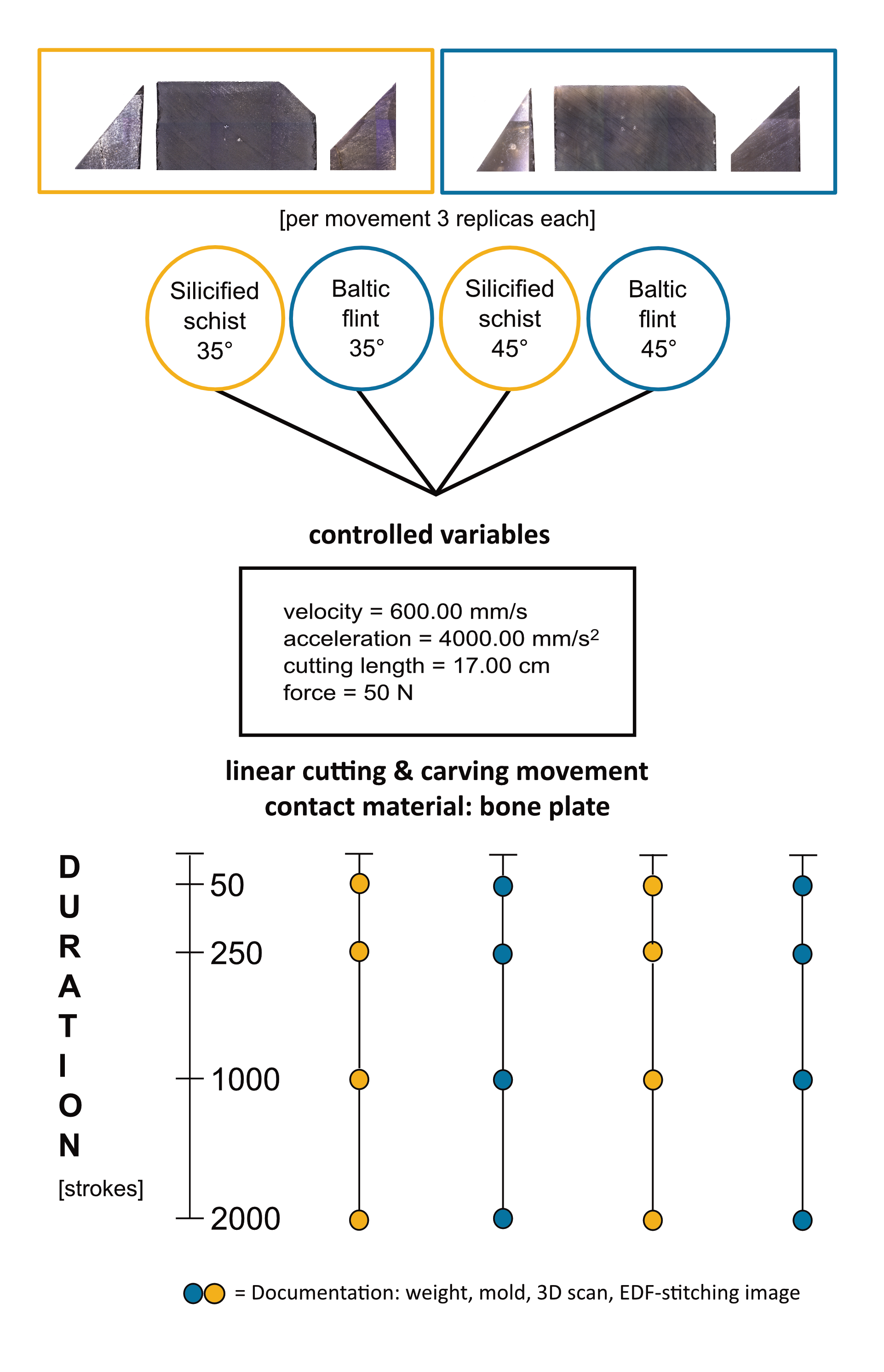
Linear unidirectional movements (cutting & carving): 2000strokes split in 4cycles .

The cycles are defined by the following number of strokes:

1strokes to 50strokes

51strokes to 250strokes

251strokes to 1000strokes

1001strokes to 2000strokes

Experimental setup

Equipment

Value	Label
SMARTTESTER	NAME
Modular material tester	TYPE
Inotec AP	BRAND
-	SKU
recorded values with the time stamps: - for each drive: position, speed, acceleration (+ deceleration) - penetration depth with distance sensor - apllied force with force sensor 1 (strain gauge sensor) - friction with force sensor 2 (strain gauge sensor)	SPECIFICATIONS

Linear movement from start point to end point:

5kg (= ~ 50 N)

170mm

600mm/s

4000mm/s2

10Hz (for each channel)

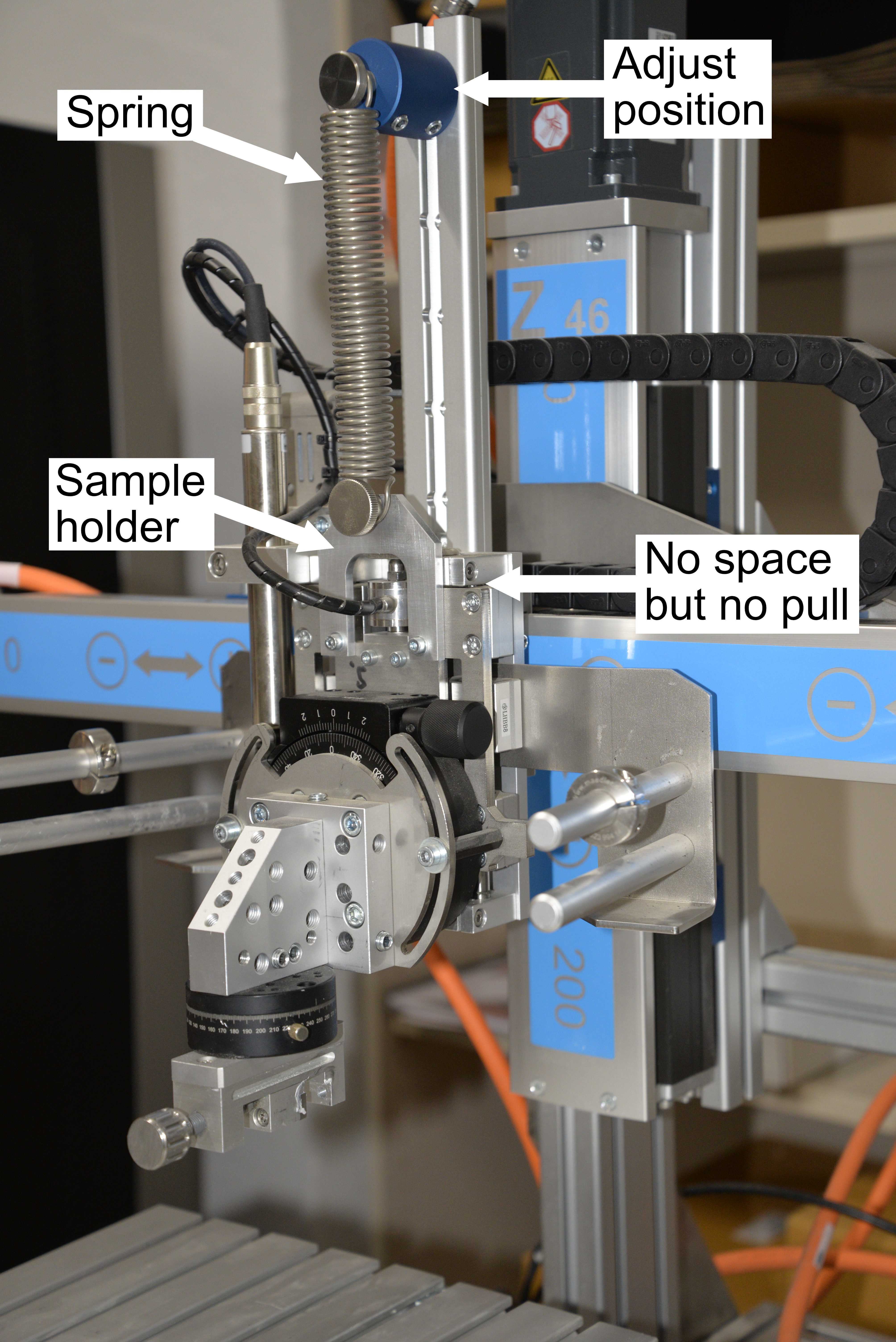
Setup sample holder

The length of the spring of the sample holder was adjusted to compensate for the weight of the sample holder (without dead weights and sample).

Adjust the position of the upper end of the spring on the rail, so that:

1. the sample holder almost touches the frame, and
2. at the same time, there should be no pull from the spring onto the sample holder.

Setup sample

The experimental standard sample (step #2) was clamped in the sample holder (SMARTTESTER) and manually oriented in all directions.

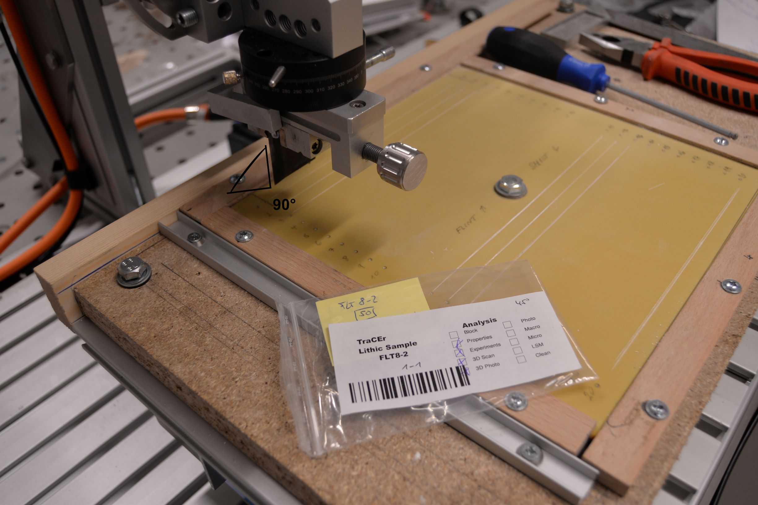
a) cutting movement

 the active edge was parallel to the contact material and the blade is mounted perpendicular to it 

(90° )

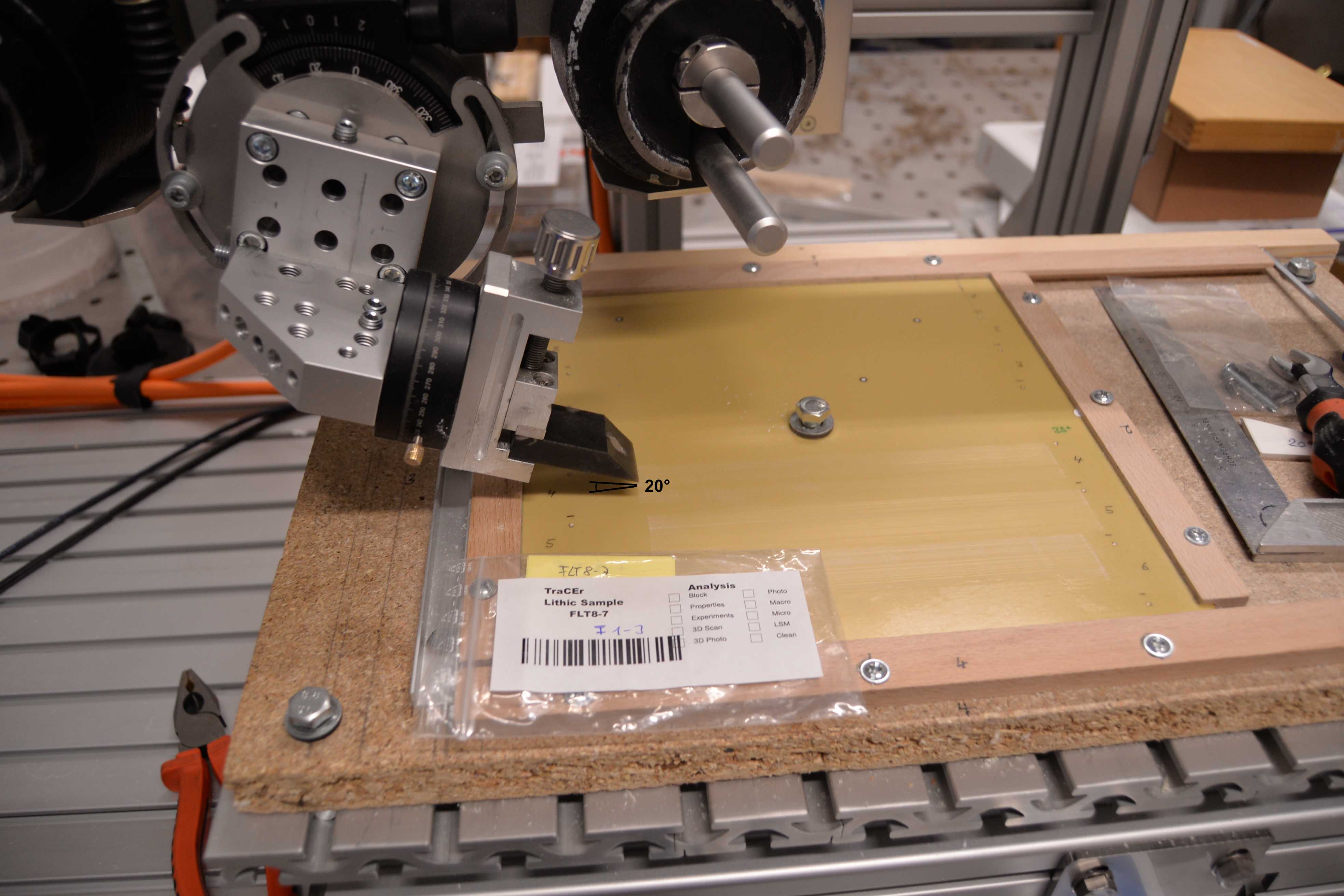
b) carving movement

 the active edge was orientated in a flat angle towards the contact material (`20°` ) 

Setup contact material

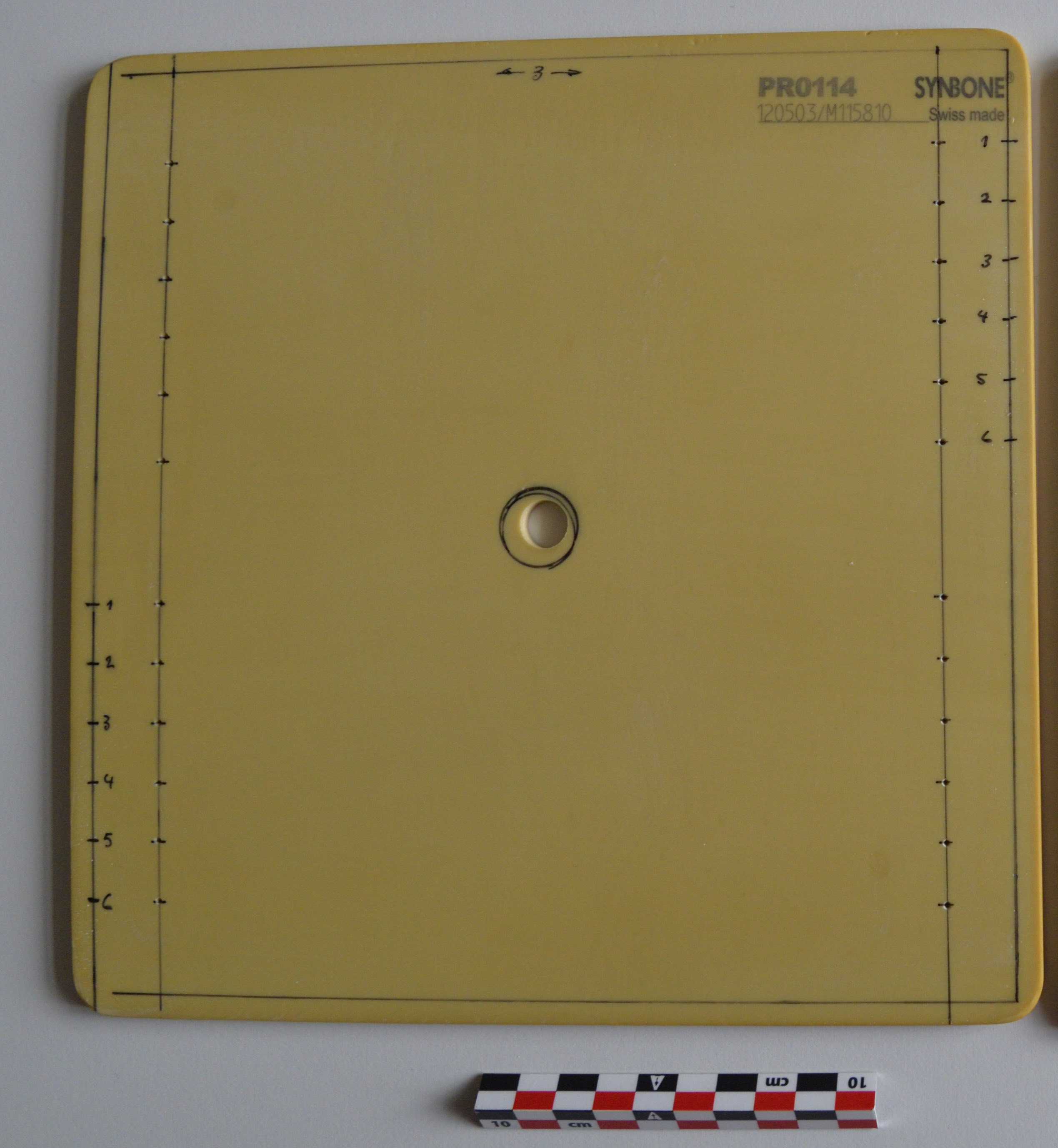
The bone plates (step #3) were clamped in a custom-made sample holder and fixed with a screw in the middle of the bone plate (see photos in step #5.2).

The plate was aligned with the X-axis.

Program cutting and carving movement

The program is identical for cutting and carving. For each sample, a new template was created (named with the sample ID and the stroke number).

a) Move down in Z-direction to start position

The z-value of the starting point was defined as follows: the sample holder on the z-drive was moved down slowly until the edge of the sample was in contact with the bone plate. 5 mm were added to the position of the z-drive in order to give the sample the possibility to penetrate into the bone plate without cutting through the 6mm-thick bone plate.

b) Move forward in X-direction 170mm (linear movement)

c) Move up in Z-direction approx. 20mm (above bone plate; no contact between contact material and sample)

d) Move backwards in X-direction to starting point

e) Loop 50 times over steps #5.4a-5.4d and export data to CSV

f) Loop 200 times over steps #5.4a-5.4d and export data to CSV

g) Loop 750 times over steps #5.4a-5.4d and export data to CSV

h) Loop 1000 times over steps #5.4a-5.4d and export data to CSV

The experiment was planned as a sequential experiment. The 2000 strokes were therefore split into four sequences (steps #5.4e-h). The experimental standard samples were documented after each sequence (step #6).

For each sequence, five CSV files were exported, one for each recorded channel:

• Penetration depth as measured by the distance sensor in the sample holder.
• Force applied (Z-direction) as measured by the force sensor in the sample holder.
• Friction as measured by the force sensor on the stage for the contact material.
• Position of the X-drive (travel range).
• Velocity of the X-drive.

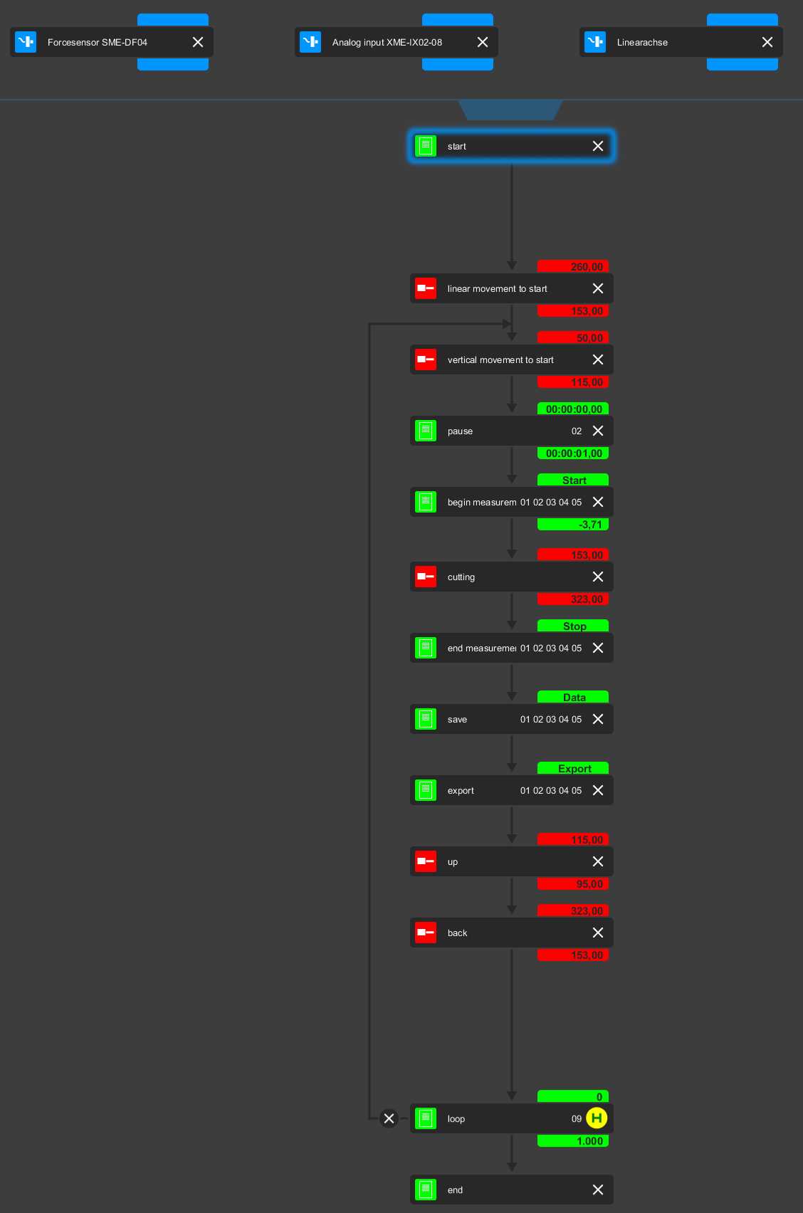
Program for sample FLT8-1 as example:

FLT8-1_cutting_template.Smart

Run program

Each sample was used for a duration of ~ 7h 0m 0s (= running time SMARTTESTER)

The following samples were used for the experiment:

Cutting 35° edge angle:

FLT8-4

FLT8-5

FLT8-6

LYDIT5-5

LYDIT5-6

LYDIT5-7

Cutting 45° edge angle:

FLT8-1

FLT8-2

FLT8-3

LYDIT5-2

LYDIT5-3

LYDIT5-4

Carving 35° edge angle:

FLT8-7

FLT8-8

FLT8-9

LYDIT5-11

LYDIT5-12

LYDIT5-13

Carving 45° edge angle:

FLT8-10

FLT8-11

FLT8-12

LYDIT5-8

LYDIT5-9

LYDIT5-10

Sample documentation

Before the experiment as well as after each cycle all 24 samples were documented in an identical way following these steps:

• cleaning with tap water and commercial washing up liquid
• weight measurement (threefold repetition)

Equipment

Value	Label
Kern PCB 3500.2	NAME
weighing scale	TYPE
Kern	BRAND
-	SKU
accuracy of 0.1g	SPECIFICATIONS

• 3D scanning of all samples (identical settings for all scans; step #1.1)
• based on the 3D models, the volume of each sample could be calculated

Equipment

Value	Label
smartScan-HE R8	NAME
3D structured light scanner	TYPE
AICON	BRAND
-	SKU
S-150 FOV, resolution of 33 µm	SPECIFICATIONS

• 3D scanning of the contact material (only before and after 2000 strokes)

Equipment

Value	Label
smartScan-HE R8	NAME
3D structured light scanner	TYPE
AICON	BRAND
-	SKU
M-450 FOV, resolution of 108 µm	SPECIFICATIONS

• optical documentation of three of the four surfaces per sample (one lateral and the two main surfaces)

Equipment

Value	Label
Smartzoom 5	NAME
digital microscope	TYPE
Zeiss	BRAND
-	SKU
PlanApo D 1.6x/0.10 objective; EDF-stitched images	SPECIFICATIONS

• cleaning the area of interest with a cotton bud with
• cleaning the area of interest with a cotton bud with
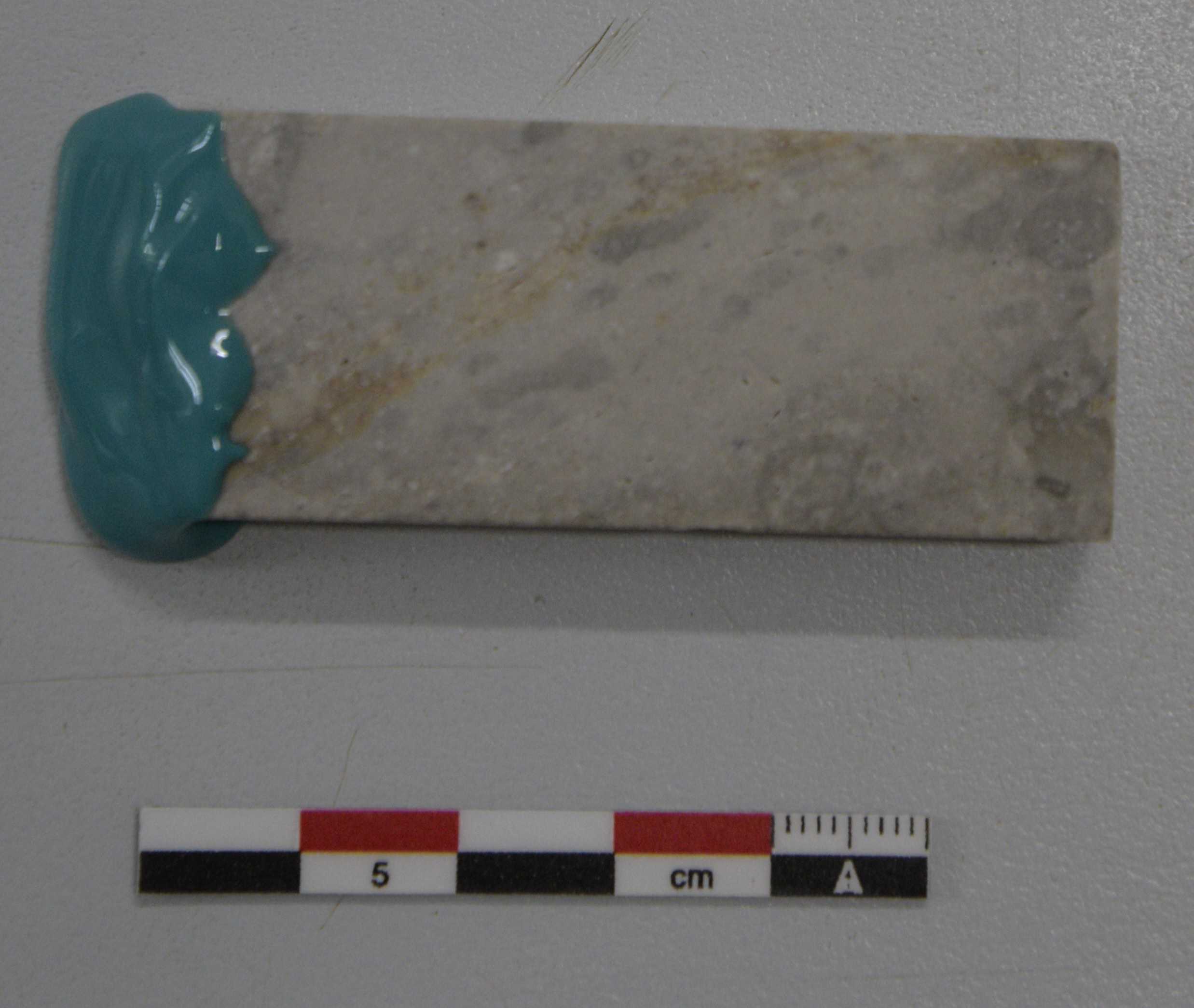
• moulding of the two main sample surfaces with

After conducting the experiment and the final documentation of all experimental standard samples, further data was acquired:

• the edge angles of the samples
• the depth and width of the cuts and scratches on the artificial bone plate

Edge angle of the experimental standard samples

The 3D models (samples + contact material) were imported as STL files into GOM Inspect and existing mesh holes were closed. 3D models were edited as described in the previously mentioned protocol:

Enhancing lithic analysis: Introducing 3D-EdgeAngle as a semi-automated 3D digital method to systematically quantify stone tool edge angle and design

Software

Value	Label
GOM Inspect	NAME
Hotfix 2, Rev. 111729, build 2018-08-22	OS_NAME
GOM	DEVELOPER
https://www.gom.com/de-de/produkte/gom-inspect-suite	LINK
2019	VERSION

Based on the closed models, the volume could be calculated.

Additionally, the edge angles of the samples after each cycle were calculated by means of GOM Inspect. To calculate the edge angle, 3D-EdgeAngle was applied again as for the archaeological artefacts (see step #1.2). Note that the parameters changed slightly ('3-points" instead of "2-lines" measuring procedure), since the "3-points" measuring procedure seems to be more suitable for simple morphologies as represented by the standard samples.

The following parameters were applied:

• "3-points" measuring procedure
• length of the line was defined with 2 mm
• as distance to the intersection the mean for distance three to six was calculated
• only sections two to eight were used

Penetration depth / dimensions of the grooves on the contact material

In addition, the contact material was documented with a Sensofar S-wide (Sensofar Metrology, Spain), a 3D optical metrology system. This way, the cuts and the scratches on the bone plate could be quantified.

Equipment

Value	Label
S wide	NAME
3D optical metrology system	TYPE
Sensofar	BRAND
-	SKU

• each bone plate was documented in four quadrants due to the limited travel range of the stage

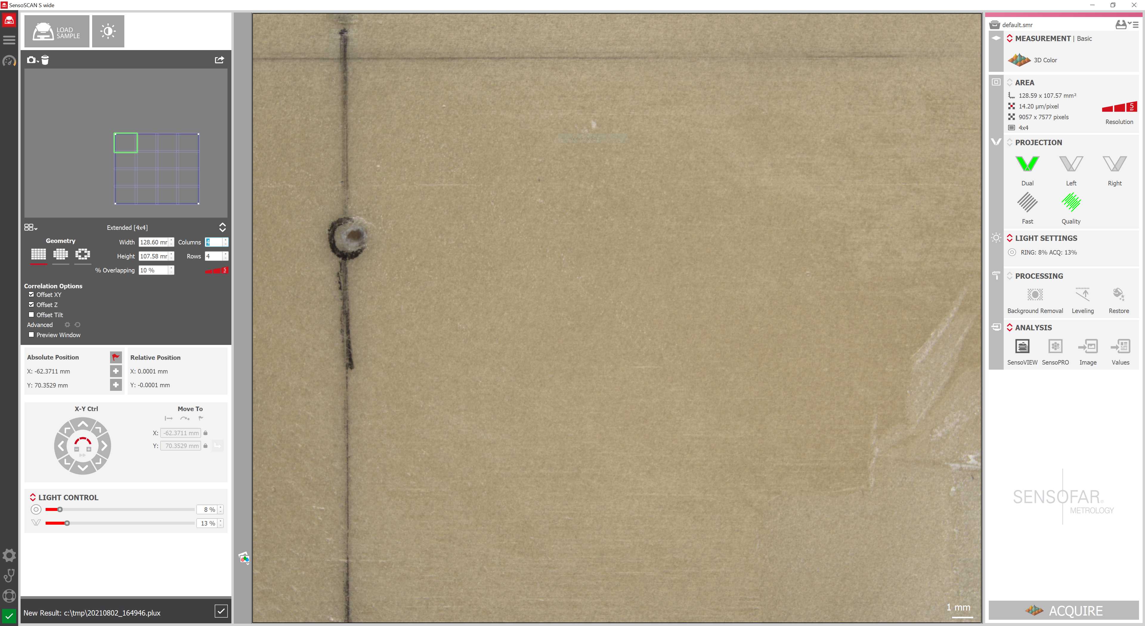
The data was processed in ConfoMap (a derivative of MountainsMap Imaging Topography developed by Digital Surf, Besançon, France; version ST 8.1.9286).

Software

Value	Label
ConfoMap (MountainsMap Imaging Tophography)	NAME
Digital Surf, Besançon, France	DEVELOPER
https://www.digitalsurf.com/de/	LINK
ST 8.1.9286	VERSION

In total, two templates were used:

a) "Patch surfaces of the bone plates acquired with the Sensofar S-wide"

An initial template was needed to patch the single quadrants together, so that the grooves are complete again. This involves levelling and aligning. Afterwards, each groove can be exported individually.

BP-I-TFE_S-wide_cutting_2000strokes_20210803_A-B.pdf

b) "Processing on single grooves"

This template extracts the topography layer of the grooves and calculates a mean profile of a series of 30 profiles. After levelling the mean profiles, the height and the width of each groove can be calculated.

BP-I-TFE_S-wide_cutting_2000strokes_20210803_FLT8-1_45deg.pdf

The ConfoMap templates for each surface in MNT and PDF formats are available in open access on Zenodo (https://doi.org/10.5281/zenodo.7565158). This also includes all original and processed surfaces.

Data analysis

The data acquired within the experiment was analysed in R.

Software

Value	Label
R Studio Desktop	NAME
The R Studio, Inc.	DEVELOPER
https://www.rstudio.com/products/RStudio/	LINK
1.1.463	VERSION

The different datasets were split in separate analyses:

a) "analysis_HLC"

This R script imports and plots the Leeb rebound hardness data acquired on the experimental standard samples (see step #2.3).

b) "analysis_EA"

This R script deals with the calculated edge angles from the experimental standard samples (see step #7.1).

c) "analysis_ST.all_sensors"

These R scripts contain the analysis of the data acquired with the five sensors connected to the SMARTTESTER (see step #5.4). However, plots concern only the data from the penetration depth.

d) "analysis_S.wide"

These R scripts deal with the penetration depth of the experimental standard samples into the contact material. The penetration depth is already part of "analysis_ST.all_sensors", but was additionally calculated with a Sensofar S-wide (see step #7.2).

e) "analysis_VW"

This R script contains the volume and the weight measurements for all experimental standard samples from before and after the experiment (see step #6).

The entire repository with all R analyses can be found on GitHub:

https://github.com/lschunk/PastHuman_StoneToolPerformance.git

and on Zenodo:

https://doi.org/10.5281/zenodo.7564605

Results

Available in open access on Zenodo:

https://doi.org/10.5281/zenodo.7564605