Bradford protein assay – Protein concentration measurement (single 595 nm read)

Prepare a solution containing 0.01% (w/v) Coomassie Brilliant Blue G-250 (e.g., B0770, Sigma-Aldrich), 4.7% (v/v) ethanol, and 8.5% (v/v) phosphoric acid as described in the next steps.

Weight 100 mg of Coomassie Brilliant Blue G-250 (e.g., B0770, Sigma-Aldrich) and dilute it in 50 mL of ethanol using a magnetic stirrer at room temperature.

In a fume hood, slowly add 100 mL of 85% (w/v) phosphoric acid (e.g., W290017, Sigma-Aldrich) to the previous solution and homogenize.

Dilute the resulting solution to a final volume of 1,000 mL with distilled water1. ¹. Filter through a Whatman No. 1 paper (or equivalent). Store at room temperature protected from light.

¹Alternatively, you can use commercially available ready-to-use reagents (e.g., 5000006, Bio-Rad).

Prepare a 4 mg/mL bovine serum albumin (BSA, e.g., A0281, Sigma-Aldrich) stock solution in PBS2. ².

Example : Dilute 6 mg in a final volume of 1.5 mL.

2 If compatible 3 , use the same solvent/buffer in which the sample to be analyzed was prepared to make the BSA standard solutions.

3 Check buffer components incompatibility with the Bradford reagent. There are several available online. For example: http://www.bio-rad.com/webroot/web/pdf/lsr/literature/Bulletin_6852.pdf and https://www.sigmaaldrich.com/content/dam/sigma-aldrich/docs/Sigma/Bulletin/b6916bul.pdf.

Check the BSA concentration in the stock solution. Read it at 280 nm in an UV-transparent cuvette and use the equation below to calculate the actual BSA concentration.

Example : If you diluted 50 µL of the BSA stock solution in a final volume of 1,000 µL and it resulted in a absorbance of 0.130, you have:

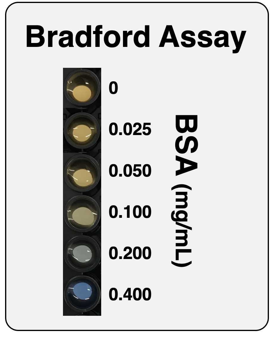
Prepare several BSA solutions at concentrations from 0.05 to 0.40 mg/mL4 using PBS (or the relevant buffer/solvent) in Eppendorf tubes. ⁴ using PBS (or the relevant buffer/solvent) in Eppendorf tubes.

Example: If your stock solution is 3.94 mg/mL, first prepare a 0.4 mg/mL (50.8 µL to a final volume of 500 µL) and then dilute it serially to 0.20, 0.10, and 0.05 mg/ mL (e.g., 100 µL of the previous solution + 100 µL of PBS).

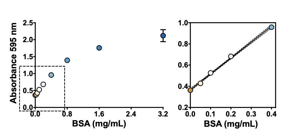
⁴Under the conditions described in this protocol, the change in absorbance at 595 nm is linear within the 0.05–0.40 mg/mL BSA range (see figure below). Note: There is another reading procedure that extends the linear range of the assay, which is to read at two wavelengths, 450 nm and 590 nm, and plot A590/A450 versus BSA concentration (see the protocol '"Bradford protein assay – Protein concentration measurement (A590A/A450 ratio)")

Dilute samples in appropriate buffer (e.g., PBS; see section/step 5) to achieve an expected concentration5 that lies within the concentration range of the standard curve (0.05–0.04 mg/mL; see section/step 7). ⁵ that lies within the concentration range of the standard curve (0.05–0.04 mg/mL; see section/step 7).

Example : Considering that rat liver contains ~100 mg protein/g wet weight, if you have a rat liver extract/homogenate that was prepared diluting the tissue sample 1:20 (resulting in ~5 mg protein/mL), you need to further dilute by a factor of least 15 (total dilution 1:300, resulting in ~0.333 mg/mL) before proceeding with the assay.

5 If an estimate of protein concentration for your tissue/cell sample is not available, test several concentrations.

Add 260 µL of water to at least three wells of a 96-well microtiter plate.

These will be the microplate reader blanks (also known as 'auto zero' or 'reference wells').

Add 10 µL of each BSA standard solution to at least three wells of a 96-well microtiter plate.

Remember to prepare a zero/blank standard, which is the buffer used to prepare the standards but with no BSA.

Add 10 µL of each sample to at least three wells of a 96-well microtiter plate.

Ideally, you should use several dilutions of the sample and check whether there is a linear response between signal (absorbance at 595 nm) and amount of sample. One convenient assay of doing it is to pipet several volumes (e.g., 1, 2, 5, 10 µL) and add it up to 10 µL with the appropriate buffer. This also maximizes the chance of getting at least one dilution of the sample within the dynamic range of the standard curve for unknown samples.

Example :

                • Dilution 1 – 1 µL sample + 9 µL buffer; 

                • Dilution 2 – 2 µL sample + 8 µL buffer; 

                • Dilution 3 – 5 µL sample + 5 µL buffer; 

                • Dilution 4 – 10 µL sample.

Add 250 µL of Bradford's protein reagent to each well containing BSA standards or samples.

If available, use a positive displacement pipette device (e.g., Multipette M4, Eppendorf) to avoid bubbles.

Do not add Bradford's protein reagent to wells containing 260 µL water. These are used just as blanks for the microplate reader.

Incubate the 96-well microtiter plate at room temperature for 5 min.

Read the microplate at 595 nm.

Read before 1 h of incubation. At high protein concentrations, precipitation begins after 10–15 minutes.

Alternatively, also acquire absorbances at 450 nm and 590 nm (see step 7).

Calculate the average absorbance for each BSA standard and samples using the absorbance values at 595 nm of the triplicates.

Build a standard curve .

Plot the average absorbance value at 595 nm on the Y- axis versus BSA concentration in mg/mL on the X-axis. Calculate a linear regression (Y = a × X + b; e.g., 'add a linear trendline' in Microsoft Excel).

Example:

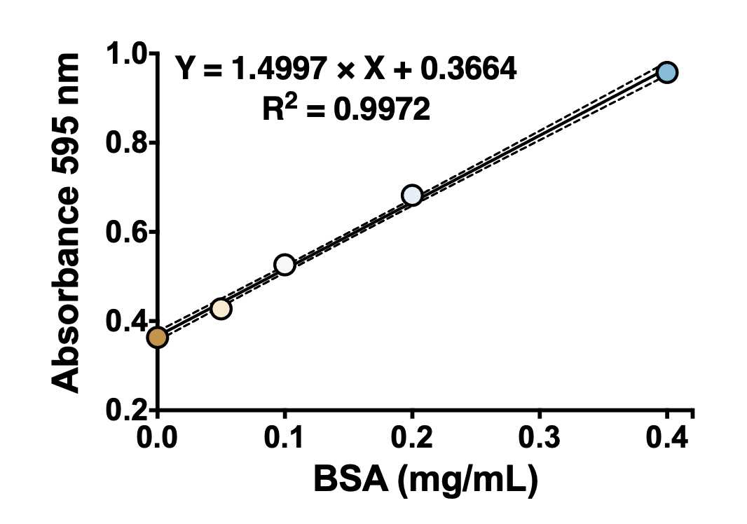
Calculate protein concentration in samples using the equation generated in the previous step.

Interpolate unknown protein concentration from the standard curve and multiply by all dilutions.

Example :

For this example (see step 15), the dilution factors are 500 (a rat liver homogenate was prepared at 1:500, w/v) and 2 (5 µL were added to the microplate and added up to 10 µL with buffer).

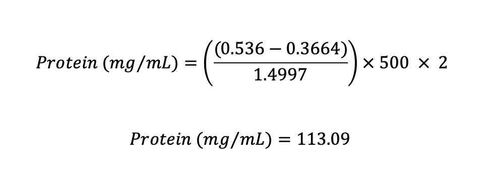
For tissues, the final result is often expressed as mg protein per gram of wet weight (mg/gww) assuming 1 g/mL. Thus, this rat liver sample used as example would have 113.09 mg/gww.