Axon tracing and node segmentation of myelinated bladder afferents in the pelvic nerve
John-Paul Fuller-Jackson, Peregrine B Osborne, Janet R Keast
Abstract
This protocol describes method for tracing myelinated axons labelled with the adeno-associated virus, AAV-PHP.S and neurofascin immunohistochemistry (to identify paranodes) in pelvic nerve of rat, using Neurolucida 360. This tracing method can be applied to various types of peripheral nerves. In rats, AAV-PHP.S has a high tropism for myelinated but not unmyelinated afferents. Cholera toxin subunit B (CTB) microinjected into the bladder was used to identify bladder afferents in the pelvic nerve. This protocol does not include details of the immunohistochemistry or procedures involving animals (viral labelling and CTB tracing). Other antibodies relevant to myelinated axons can be used instead of neurofascin.
Steps
Image acquisition
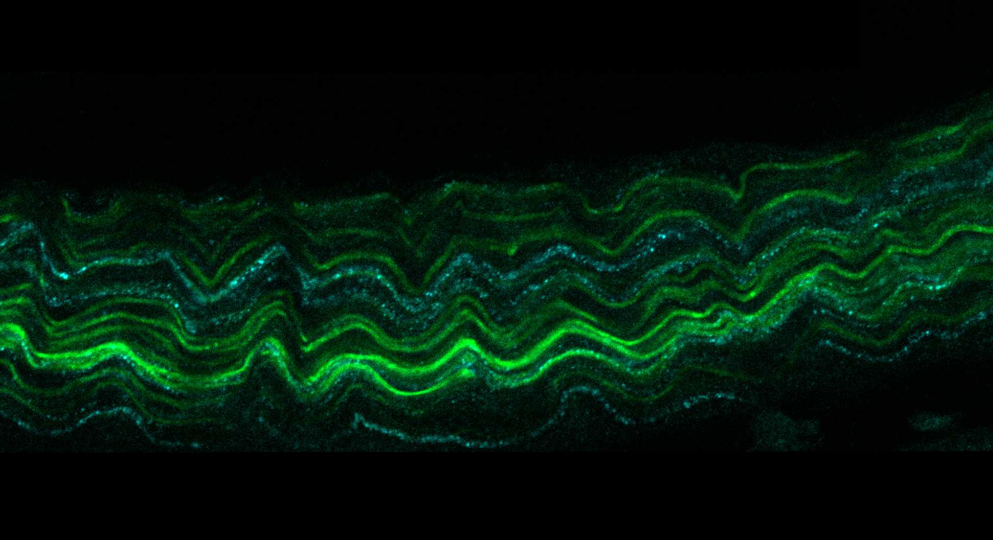
On a confocal microscope, scan the nerve fascicle with sufficient magnification and resolution to achieve a voxel size of at least 0.099 x 0.099 x 1 μm (XYZ). This will require multiple tiles acquired with 10% overlap.
Image pre-processing
Stitch together the tiled image stack dataset into a new single image.
Convert the stitched image to JPEG2000 (JPX) using MicroFile+.
Software
| Value | Label |
|---|---|
| MicroFile+ (RRID: SCR_018724) | NAME |
| MBF Bioscience | DEVELOPER |
Opening file in Neurolucida
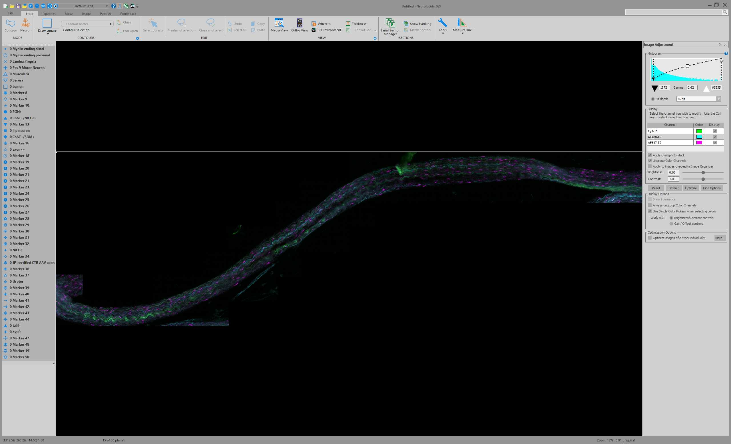
Open the converted nerve JPEG2000 dataset in Neurolucida 360 .
Software
| Value | Label |
|---|---|
| Neurolucida 360 | NAME |
| MBF Bioscience | DEVELOPER |
| https://www.mbfbioscience.com/neurolucida360 | LINK |
| v.2020.1.1 | VERSION |
Thoughout all the subsequent Steps, save progress. This will prompt a saving of the JPEG2000 (if display settings were altered) and the saving of a data file. Choose .XML as the file type for saving the data file. Keep the .XML in the same file location as the associated JPEG2000.
Identification of specific axon classes
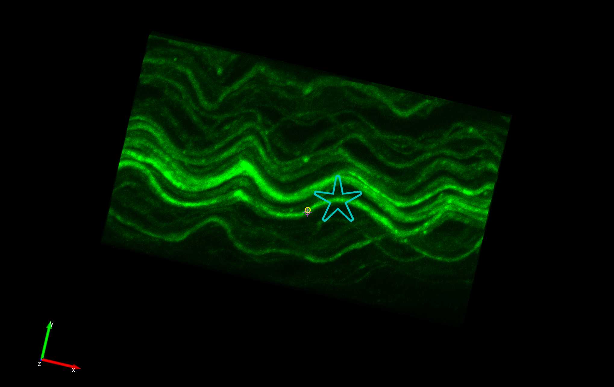
In the 2D view, zoom in to the nerve dataset until individual axons can be discerned.
Search the nerve fascicle by moving around in XYZ for myelinated (AAV-PHP.S+) bladder (CTB+) axons and mark them with a marker from the panel on the left.
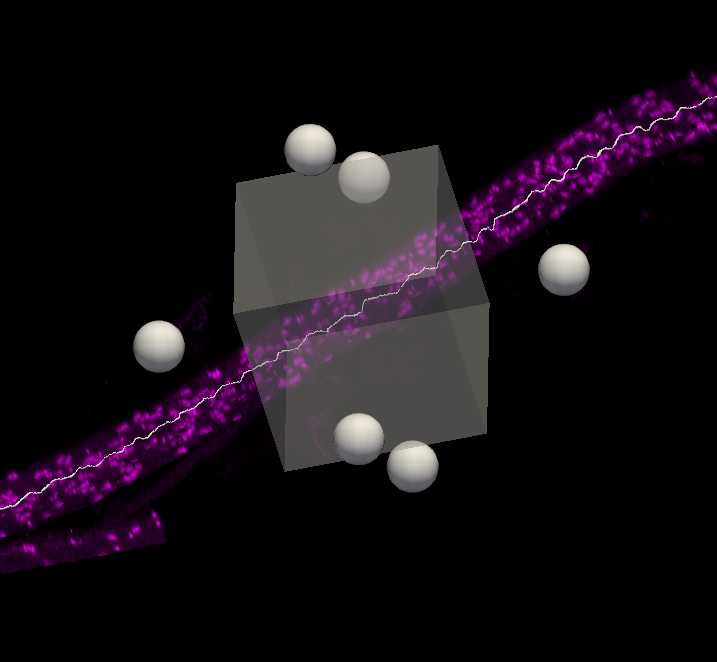
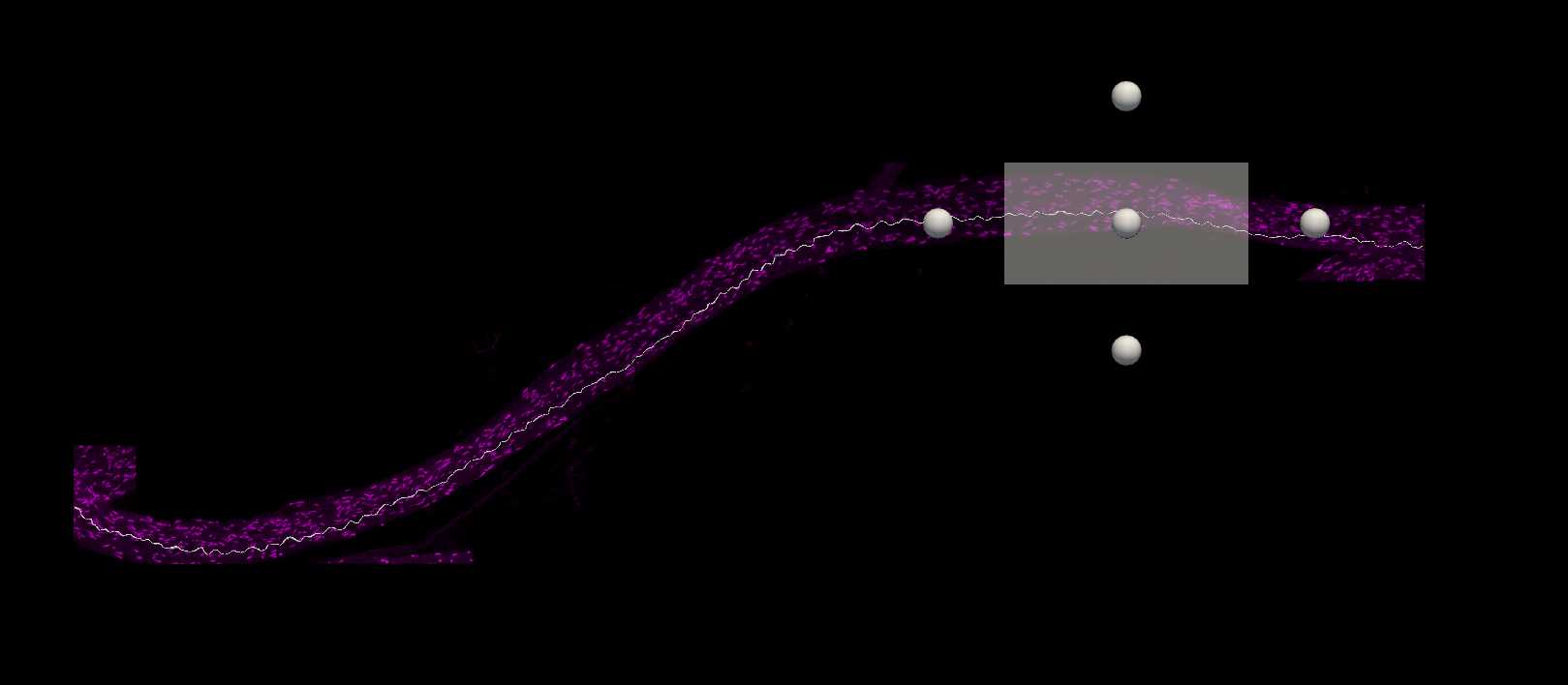
Subvolume 3D viewing of axons
Open the 3D Environment to view the dataset in 3D.
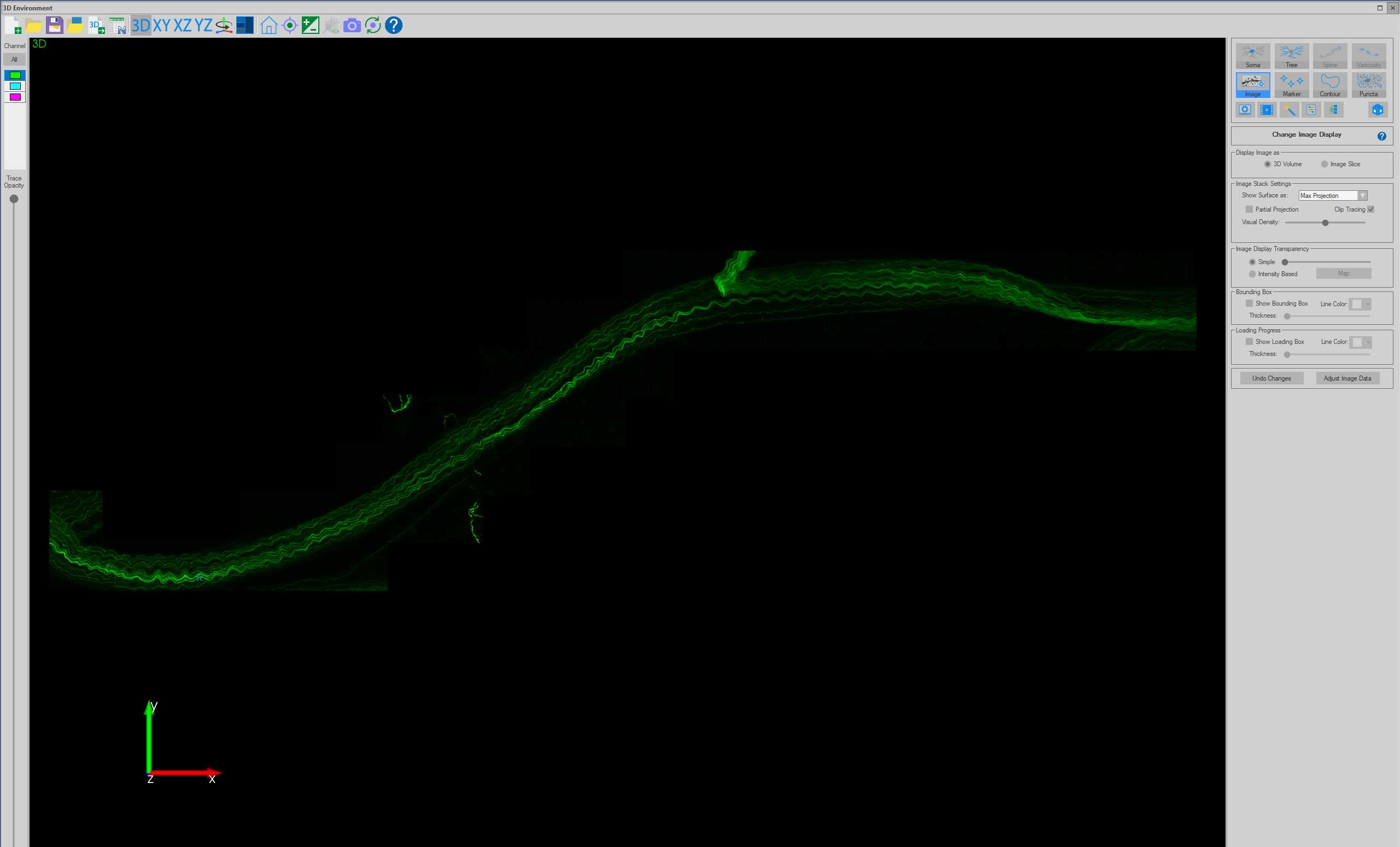
In the top right-hand menu, click on Subvolume .
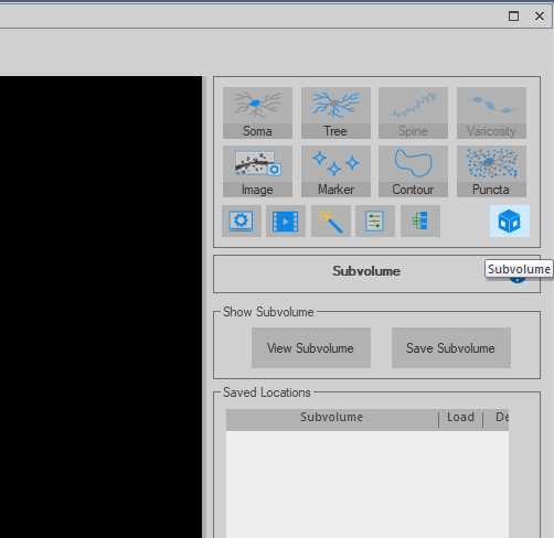
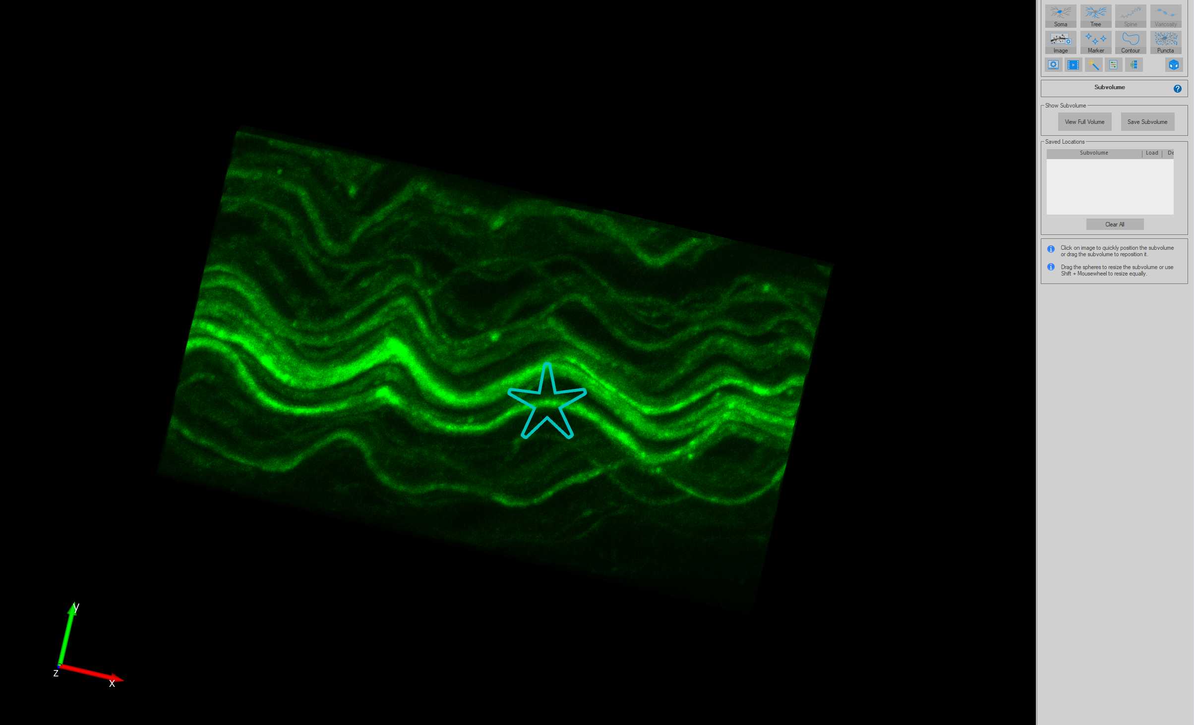
Move the Subvolume region to cover one of the markers established in Step 6.
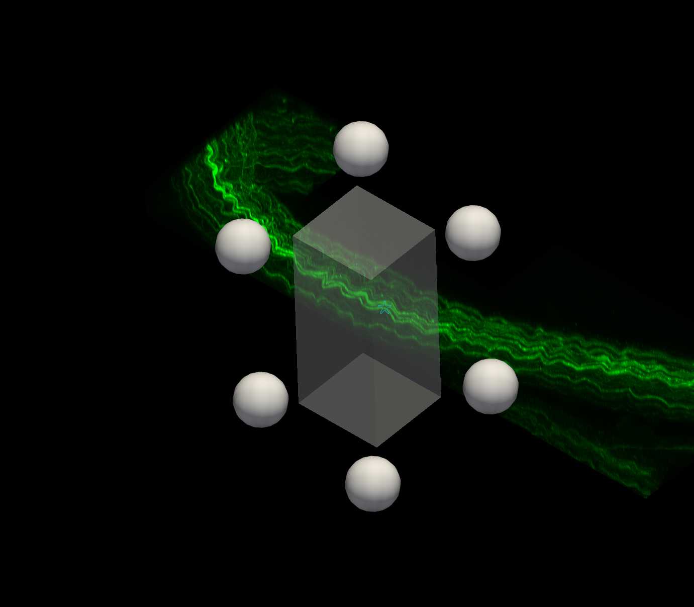
Click View Subvolume to view only the region selected.
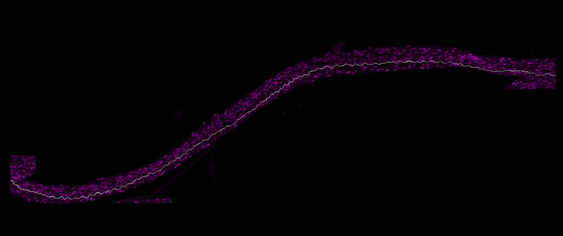
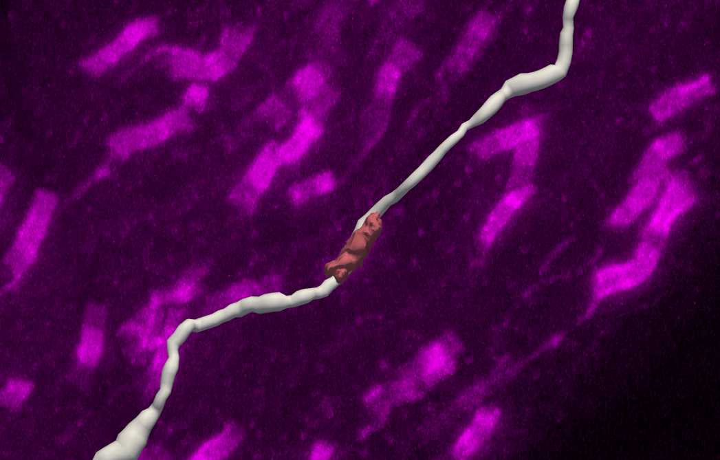
Tracing axons using AAV-PHP.S fluorescence
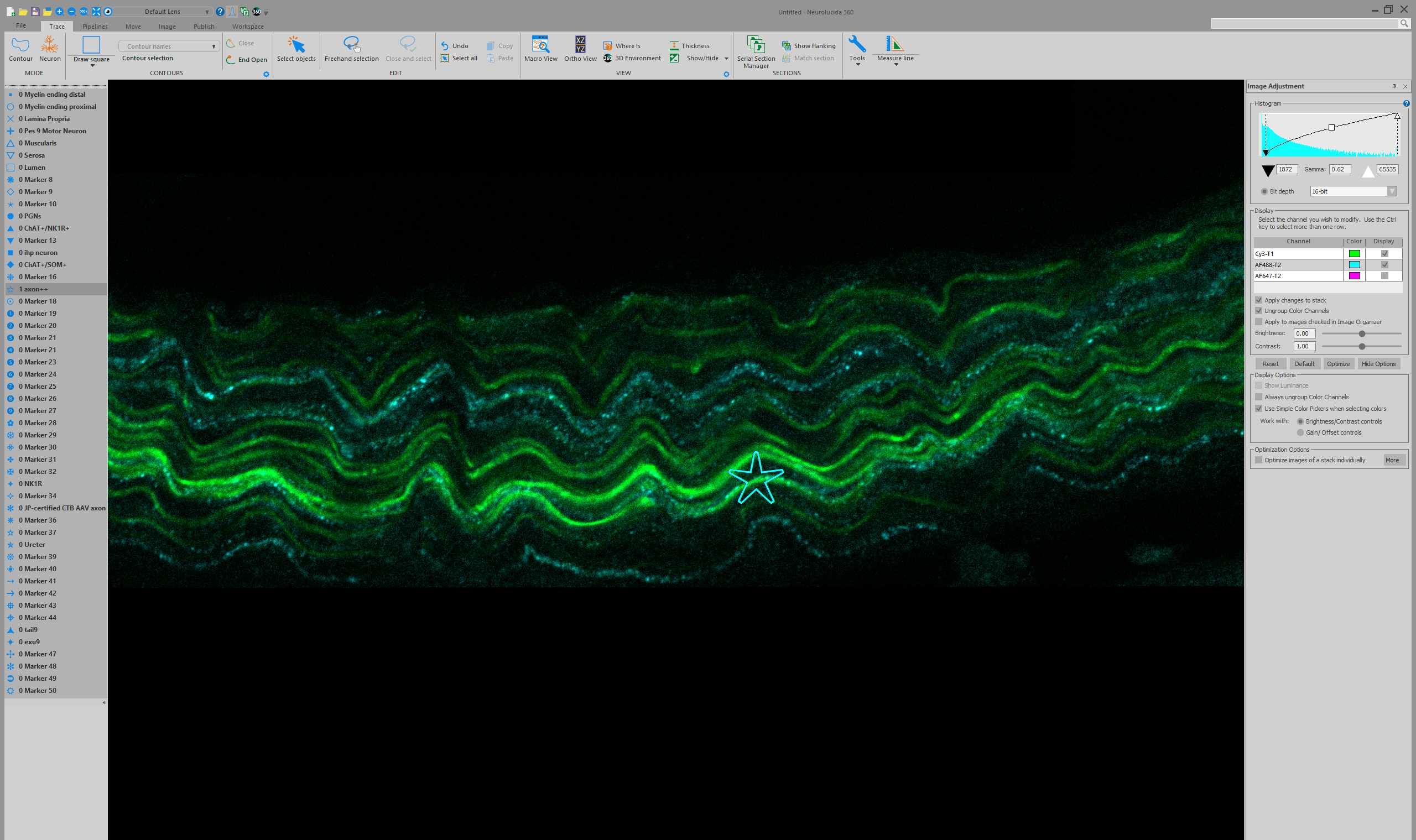
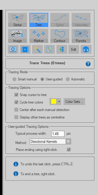
Using the channel in which the AAV-PHP.S fluorescence was acquired, start the tracing by clicking on Tree in the right-hand side panel. Select User-guided and under the User-guided Tracing Options select Directional Kernels as the Method .
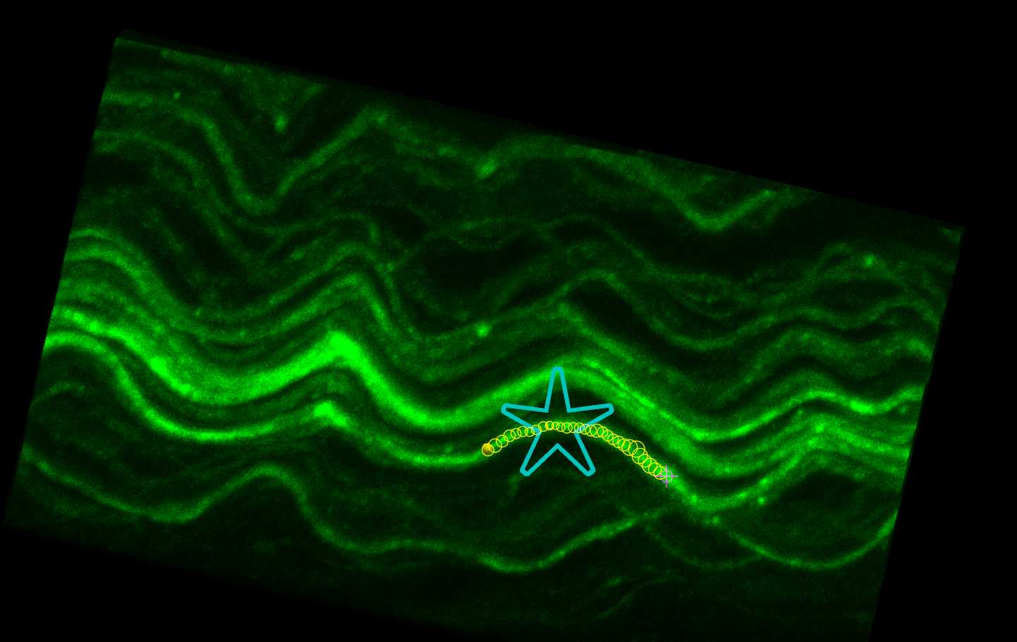
Move the cursor onto the desired axon to be traced in the Subvolume image stack, a small circle should appear on the axon of approximately the same diameter as the axon. This is the starting point of the tracing. Left click to start tracing.
Move the cursor along the axon. A string of circles of the axon diameter should follow the cursor, these are individual points of the axon tracing. Go as far as possible without the points deviating from the axon. Left click to confirm points, current position will become the new start position.
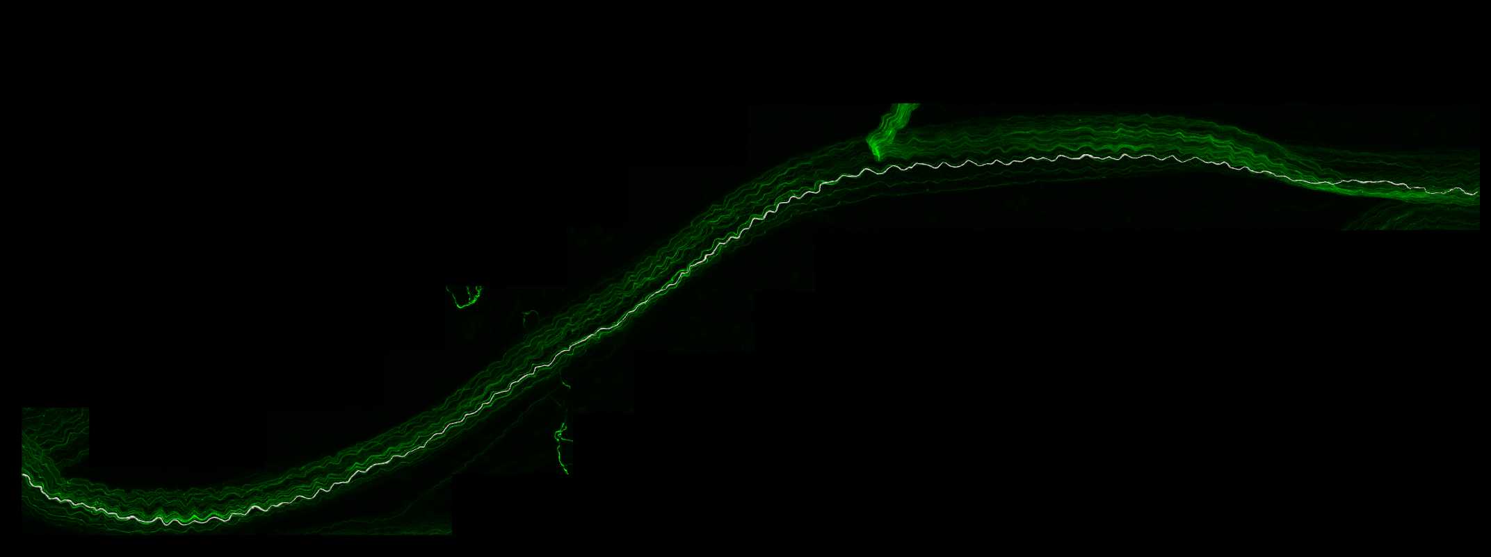
When the tracing approaches the edge of the Subvolume region, the Subvolume region will automatically shift in the direction of the tracing to allow for seamless tracing of axons without the need to view the entire image stack. Continue tracing until the end of the axon (or when the axon cannot confidently be traced).
Paranode segmentation on traced axons
Swap the displayed channel to that in which the Neurofascin immunofluorescence was acquired.
As in Steps 8 and 9, select a region of the image to view via Subvolume .
In the Subvolume region, search along the traced axon for Neurofascin labelling that completely overlaps with the axon. Move the image to see the paranodes from multiple angles to ensure correct identification of nodes on the axon. Move the Subvolume region along the axon progressively until a paranode is found.
.")

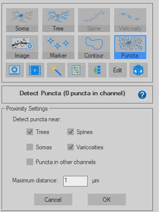
With a paranode identified, in the right-hand panel click on Puncta . Keep the Detection Method set to Automatic . In Detection Settings , select Detect based on proximity and click on Settings...
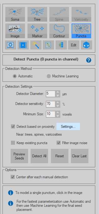
Under Proximity Settings make sure Trees are ticked and set the Maximum distance to 1 µm. Click OK.
Left click on the paranode in the image to segment that specific paranode. This will create a Punctum that represents the paranode.
If the detection fails, this is unlikely to be a paranode along the axon (too far away). Sometimes Detector Sensitivity can be adjusted for signal that is not being detected but is clearly along the axon.
Continue inspecting the dataset for paranodes along the axon, moving the Subvolume . For each paranode identified, re-select Puncta and repeat Step 20 to segment the paranode.
Axon and paranode data extraction
To extract data, open the .XML file created by Neurolucida 360 in Neurolucida Explorer .
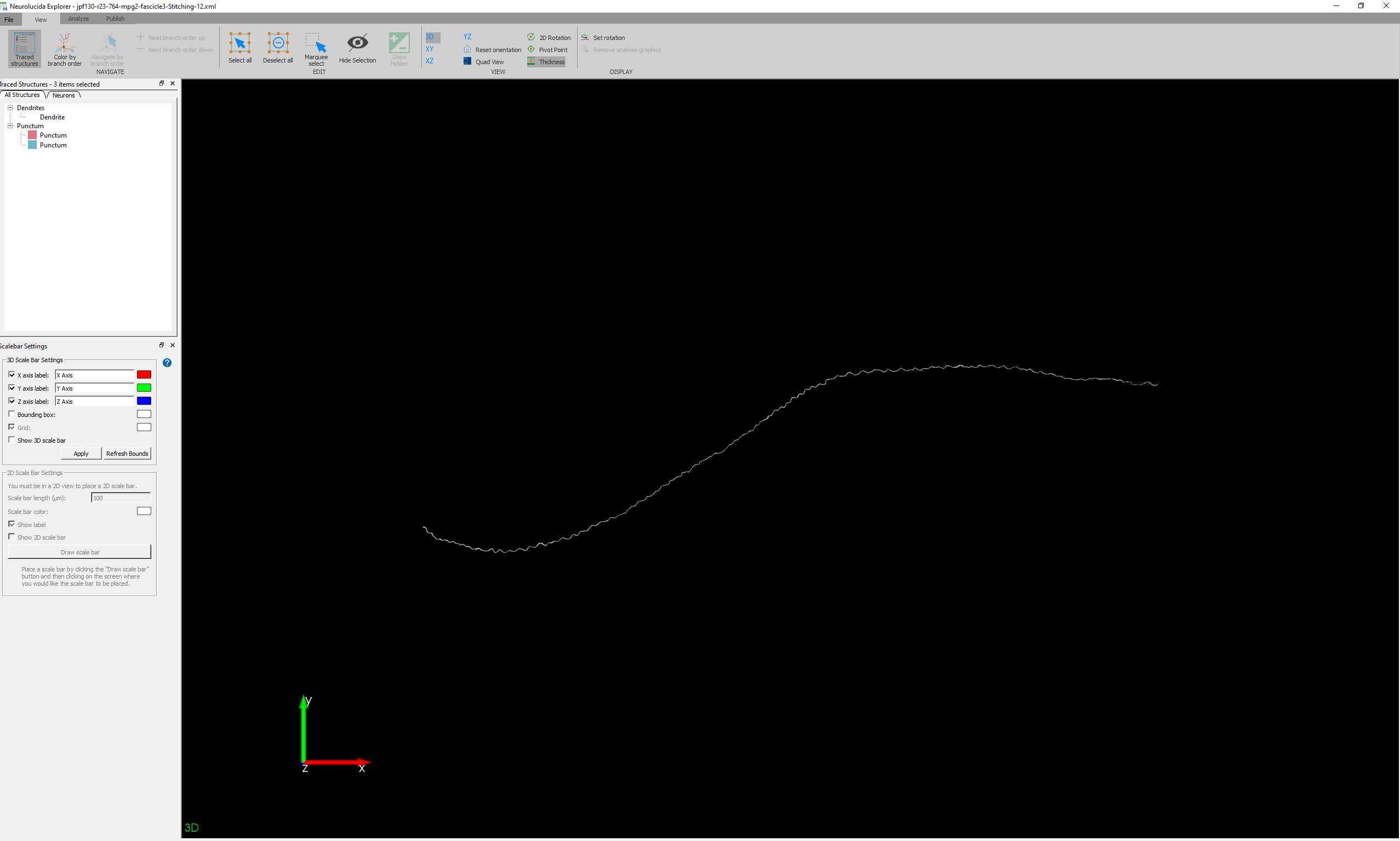
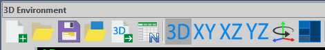
This can be done directly from the 3D Environment of Neurolucida 360 by clicking on the icon that looks like spreadsheet with a superimposed 'N'. This will open the current .XML in Neurolucida Explorer .
Software
| Value | Label |
|---|---|
| Neurolucida Explorer | NAME |
| MicroBrightField Bioscience | DEVELOPER |
| https://www.mbfbioscience.com/neurolucida-explorer | LINK |
Select all the axons and punctum, either manually or by clicking Select all .
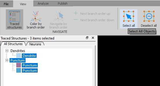
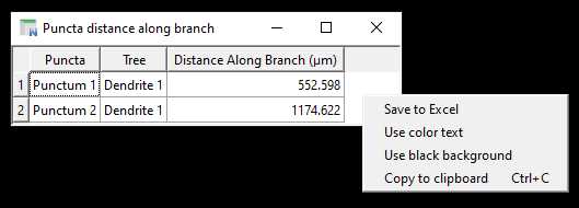
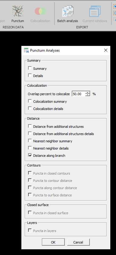
Click on Punctum to bring up the Punctum Analyses panel and select Distance along branch . Click OK.
A window titled Puncta distance along branch will appear with an interactable spreadsheet listing each Puncta (paranode) and its distance along the Tree (axon). To export this table, right click and select Save to Excel to save a .CSV.