Modular Reconstruction and Co-registration of Imaging from Implanted ECoG and SEEG Electrodes

Retrieve Images

When retrieving imaging as DICOMs, you can download the entire imaging series or just the sequence of interest, whichever is easiest for your setup. If there is not a T1 MRI with high enough resolution, a T2/FLAIR image with good resolution can supplement (but not replace!) the bad T1 in the FreeSurfer reconstruction process (see Step 2.2).

Download pre-op MRI imaging. MRI requirement:

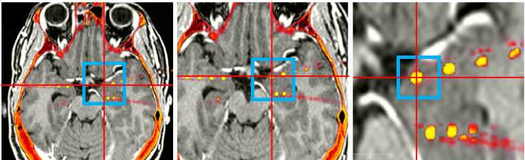
• T1 (MPRAGE, SPGR, Ax T1 NAV, ect.) with as many slices as possible, good resolution between grey and white matter, and ideally without contrast (Step 1.2, Panel A).

Download post-op imaging.

• Ideally post-operative CT (Panel C), although post-operative MRI (Panel B) works as well.

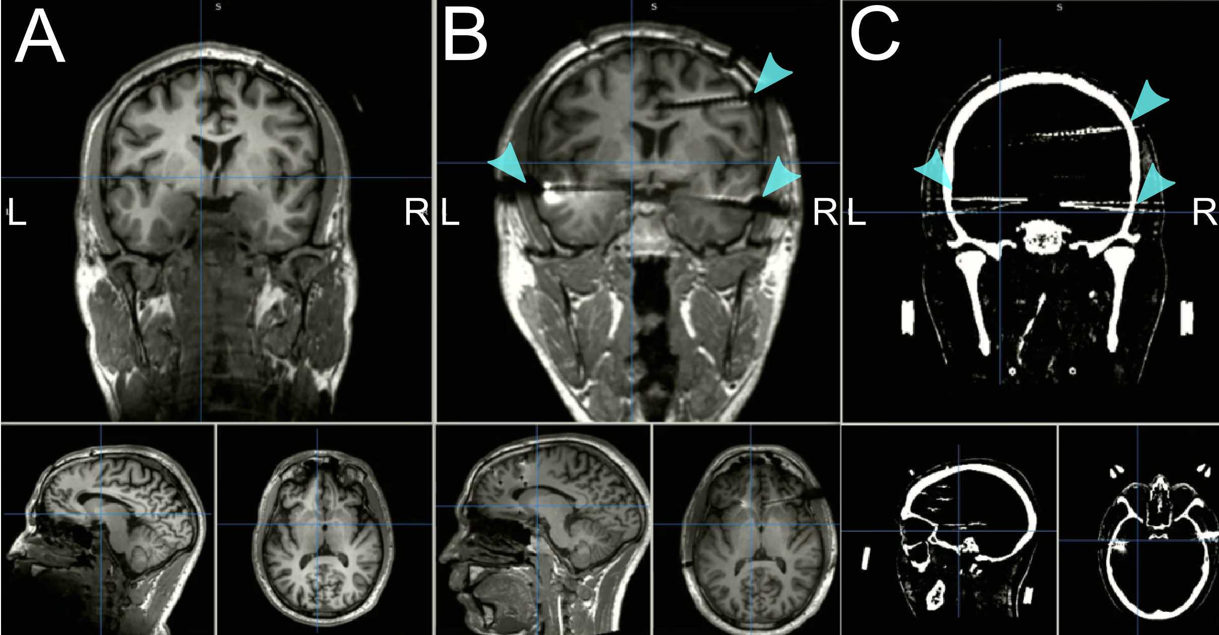
Convert imaging to compressed NifTI (.nii.gz).

• (Recommended) Download Mango, open image or images folder, "Files > Save As" into a compressed NifTI (nii.gz).
• Alternatively, use FreeSurfer’s mri_convert function to create NifTI files for both MRI and CT sequences of interest.
• If you run into any issues, dcm2niix may be a good backup program for converting sequences (see Materials).

FreeSurfer Output

Once

your imaging scans are selected, move the pre-op NifTI file into the folder required by FreeSurfer installation (usually somewhere like ~/home/freesurfer/subjects). During this step, you will open a terminal (right click and select “Open Terminal”) and run the commands which make all the 3D files, cortical parcellations, and subcortical segmentations of the input brain. From here on, any instance of “id##” is the name and number of the subject you are currently running through the pipeline. You must replace every “id##” with your subject name .

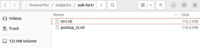
Make a ../freesurfer/subjects/ id## folder and move the pre-op NifTI file into this folder

Open a terminal window and change directories within it to where you placed the mri.nii.gz file (see APPENDIX I for more info on using the terminal). Type these four commands, pressing enter after each command:

tcsh
setenv SUBJECTS_DIR ${PWD}
setenv SUBJECT id##_SurferOutput
recon-all -all -s $SUBJECT -i mri.nii.gz
```<img src="https://static.yanyin.tech/literature_test/protocol_io_true/protocols.io.5qpvornedv4o/k3zsbxz3722.jpg" alt="" loading="lazy" title=""/>

  

If you want to run the recon-all for a patient with grids and strips ECoG, you will need to run it with the "-localGI" flag at the end of the first command. You will also need the Image Processing Toolbox from MATLAB:

recon-all -all -s $SUBJECT -i mri.nii.gz -localGI

recon-all -all -s $SUBJECT -i mri.nii.gz -T2 T2.nii.gz -T2pial

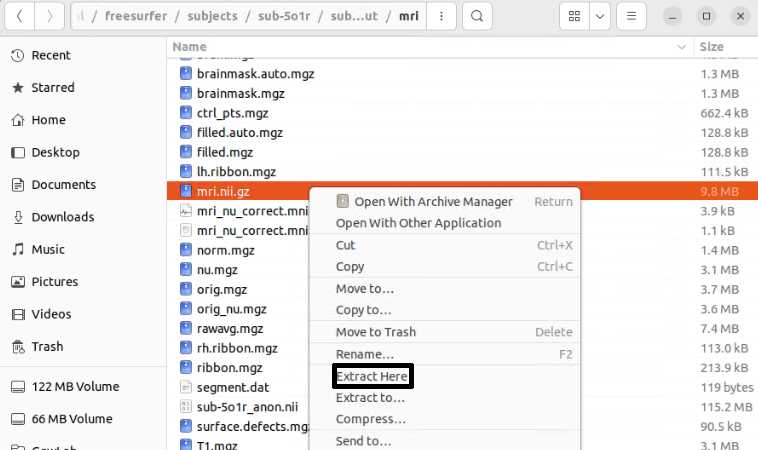
Once finished, copy the pre-op NIfTI file into the _id##SurferOutput/mri folder and extract the file so the mri.nii(extracted) is in the mri folder. The extraction step can involve unzipping the file using any extraction software (e.g., WinZip, Bitser), or by right-clicking and selecting some form of “extract”.

If you wish to have a better sub-thalamic segmentation, you can use a segmentation script supplied in versions of FreeSurfer 7.2 and newer. Run the first three commands from the recon-all (Step 2.2) and then run:

segmentThalamicNuclei.sh $SUBJECT
```This step only takes a few minutes, typically.

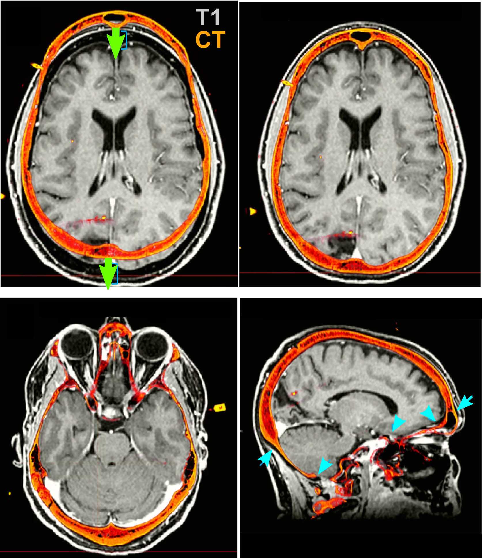
MRI/CT Co-Registration with Freeview

Open a terminal, type the following command, and press enter. A window will pop up:

freeview

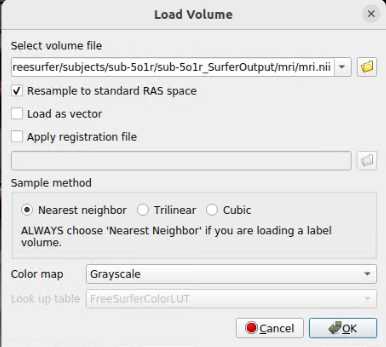
Load the pre-op file:

• Click on File > Load Volume. A dialog box will appear. Select the pre-op NIfTI volume file in the browser. Select the “Resample to standard RAS space” checkbox to reorient to RAS coordinates. Hit “OK”.

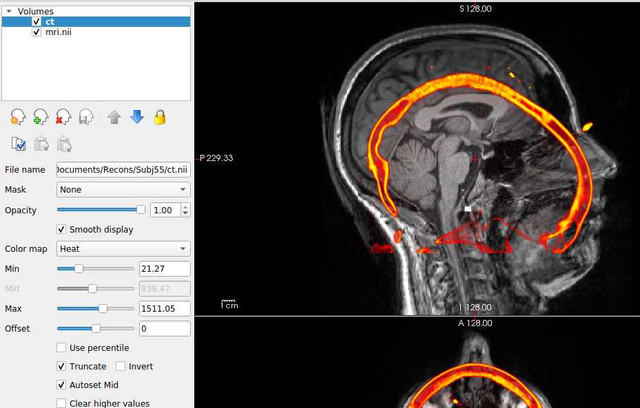
Load the post-op file:

• Click on File > Load Volume. A dialog box will appear. Select the post-op NIfTI volume file. Choose a color map (at the bottom of the box) to best visualize the electrodes and skull. We suggest the "Heat" color map. Hit “OK”.
• Further suggested adjustments: 9. Using side selection pane, adjust the min, mid, max, and offset values to best see the outline of the skull (with the post-op volume selected!). ii. If using a post-op CT, select the “truncate” and “smooth” check boxes in this panel to remove noise in the image.

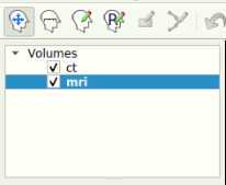
With the post-op imaging highlighted in the top left “Volumes” window (do NOT select the MRI to transform!), align the skull outline in the post-op imaging with the black of the MRI using the transform tool:

• At the top, select Tools > Transform Volume to open the tool

There are four options: Rotate, Translate, Scale, and Flip. We suggest that you practice rotating and translating the selected volume with the sliders to get a sense of what each one does and feels like to move. Scaling and Flipping are rarely ever needed.

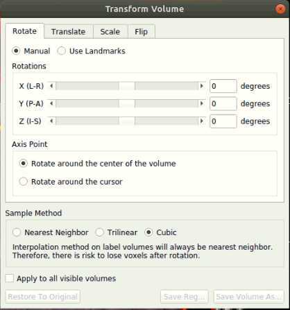
Transform the volume until the post-op image aligns with the pre-op image.

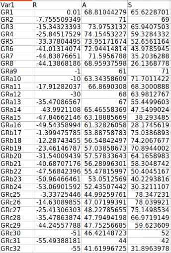
Identifying RAS Coordinates

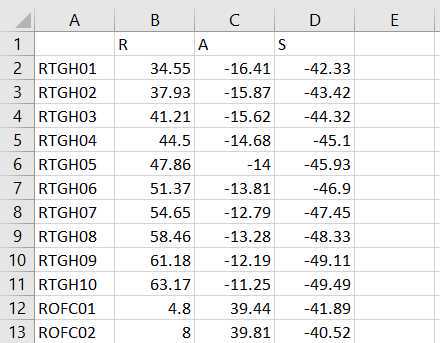
Make an excel spreadsheet named id## _id##RAS.xlsx with 4 columns and n+1 rows, where n is the number of electrode contacts for which you find locations in Freeview. The first column has the names of each electrode contact, and the other three are for the three axes: R, A, and S. (Right, Anterior, and Superior)

Highlight the pre-op mri volume layer in the top left in Freeview

Use the crosshairs/cursor to locate each electrode. Click on the center of the contact in all three views to ensure that you have the most accurate location

Write down the RAS from the TkReg RAS (mri) row at bottom of screen for each electrode contact. A video example of this for sub-03ti is in the Materials section.

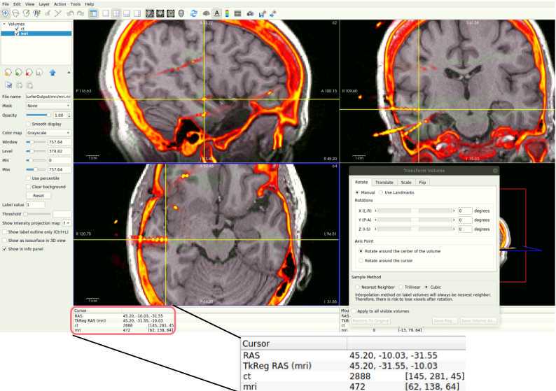
Once all RAS coordinates for all electrodes have been located, check to ensure that the orientation of the coordinates is correct using this test: look at the RAS coordinates section in Freeview (Step 4.4 Figure, zoomed portion). The R, A, S numbers (the first, second and third numbers in the Freeview TkReg RAS row) should increase positively in the right, anterior, and superior directions, respectively. If they do not, you must account for this in coordinate transcription. There are 3 options for each of the coordinates, R, A, and S:

1. All values are in the correct orientation. Nothing additional needs to be done once you write down the value from Freeview.
2. Some of the values are switched (e.g., R may be in the S position). Test this by moving the cursor in each of the three directions and making sure the value in the correct spot changes in RAS instead of ARS or SAR. For example, moving the cursor towards the anterior of the image will result in the second value in the RAS field changing.
3. Some of the values could be inverted. This means the RAS values are in the correct order, but they may be flipped. For example, if the R value decreases when you move the cursor to the right and increases when you move the cursor to the left, then R values are inverted.

Just account for these changes in the final RAS excel sheet before moving forward. Multiply inverted columns by -1 or shift columns which were switched in the original Freeview.

Snapping the Grid to Brain Surface (only applicable for grid/strip (ECoG) electrodes. If your subject has exclusively depths (sEEG), skip to next section)

You should create a directory in which you place each subject’s folder. We will call this the working directory (wd).

Create an id## folder in the wd containing:

• RAS coordinates in an Excel spreadsheet
• SurferOutput folder for the patient

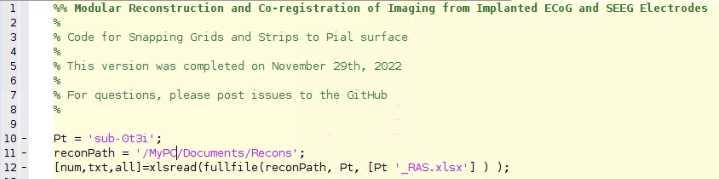
For each patient, make a new copy of “ idxx idxx_Snap_to_Grid.m ” from the Protocol_Snap_to_Grid.m code file located on the GitHub page. This isn't necessary, just a recommendation.

Change the Pt (line 10) and the reconPath (line 11) variables to be the patient's name and the path to your wd folder, respectively. Also, ensure that the GitHub code and iELVis code are on the path.

Next, you must create a variable which has each electrode’s RAS coordinates. Please look in the Protocol_Snap_to_Grid.m for an example of how this is done. You can partition them up as whole electrodes or break them down into strips. For example, if you have an 8x8 grid, we usually break it down into eight 1x8 strips. Each strip will usually be handled by the algorithm better than the whole grid, though you can experiment with keeping them whole. Start the counting of the RAS_coords at 1, as in this example, and not at 2, as in the RAS file itself.

Ensure the side variable (line ~40) at the top of the next section is set to the correct hemisphere (“l” for left, and “r” for right). If you have grids and strips on both hemispheres, you will have to run this through twice, once for each side. Generally, a patient should only have grids and strips on one side, so only run this on the hemisphere on which the electrodes are placed.

Run each of the snap2dural_energy_customized(...) lines (lines 45+) for each electrode or grid/strip segment.

_gr#coor_snapped are the newly snapped coordinates.

When you run this algorithm for each electrode RAS variable you made, you will see a 3D projection of the electrodes as they snap themselves to the brain’s surface. You should watch each of these carefully as they will tell you if the algorithm is functioning as desired. The electrode contact points should be moving along a relatively straight line to the brain’s surface ( FIG ii ). They shouldn’t criss-cross or come out of their expected alignment ( FIG i ). If they do, decrease MaxIter (around line 45) in the snap2dural_energy_customized.m file. This can involve a lot of trial and error, but generally, if it doesn't work at default (MaxIter=50), then you should decrease it to <5. You can also check the Tips for Customizing iELVis Code Package.docx file for some help (see Materials).

Once you have the snapped coordinates, run the next two MATLAB sections which overwrites the input RAS file to have the newly snapped coordinates. This section also makes a backup so you can redo the snap if need be ( _id##RAS_bkp.xlsx ). Make sure the RAS_coords_new variable (~line 55) has the electrodes in the same order that they were in the original RAS file. For example, if the input RAS has order of electrodes: GR1-64, RAH1-16, RPH1-12, STS1-16, then you should have the output _{rasElecName}coor_snapped in the same order in the RAS_coords_new variable. Plot the newly made snapped RAS and examine it carefully to ensure it is accurate. This can be done by running the first two sections of the imaging code (Step 6) with the newly snapped RAS.

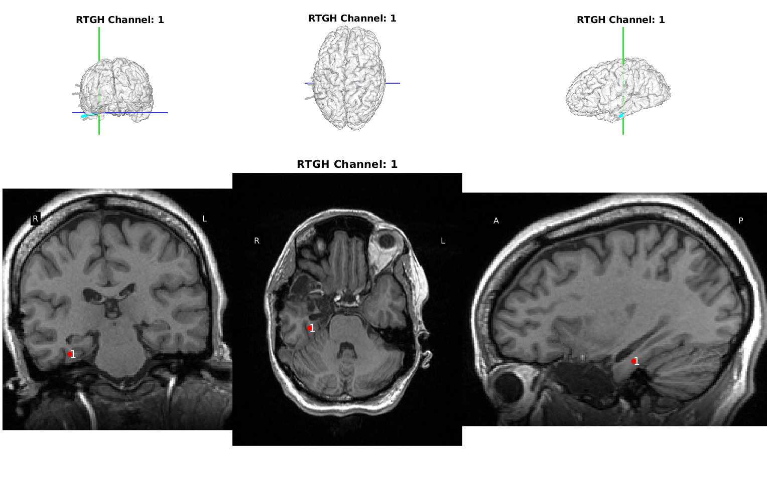
Creating Images of MRI with Electrode Overlay

Create an id## folder in the wd containing:

• RAS coordinates in an Excel spreadsheet
• SurferOutput folder for the patient. The mri.nii file should be in the surferoutput/mri folder.
• If you are only making 2D visuals (i.e., no SurferOutput), then you must place the mri.nii in this subject folder as well

This section will work if you have converted your files into the BIDS format (Step 8).

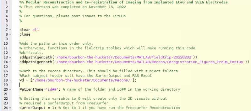
Open “Protocol_recon_code” (located in Coregistration_Figures_PreOp_PostOp) and change wd (line 18) to the path to your wd and PatientName (line 20) to your id##. If you have not run the FreeSurfer section (Step 2), then set surferOutput (line 24) to 0, and you will only get 2D visuals.

Add the paths to the Fieldtrip toolbox and GitHub pipeline code on lines 13 and 14.

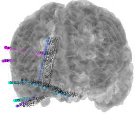
Run the first cell of the code, which sets variables, loads data into MATLAB, and reads the SurferOutput files you made in Step 2 to create a 3D image of the brain

Create 3D image with electrodes by clicking "Run Section" in the second cell.

• To change opacity, change number after “facealpha” (lines 136, 138). The range is 0-1, where 1 is fully opaque. For depths, 0.3 looks the best, while 0.9-1 is best for grids/strips.
• If need be, RAS locations can be transformed on line 186-188. This is only necessary if snap does not work well.

Creates Images which re-slices the MRI to capture the plane of the electrode with the coronal view along the entire depth electrode (skip for grids/strips) by clicking "Run Section" in the third section. This section involves producing coronal slices which are angled along the length of the depth electrode to ensure that every contact is shown.

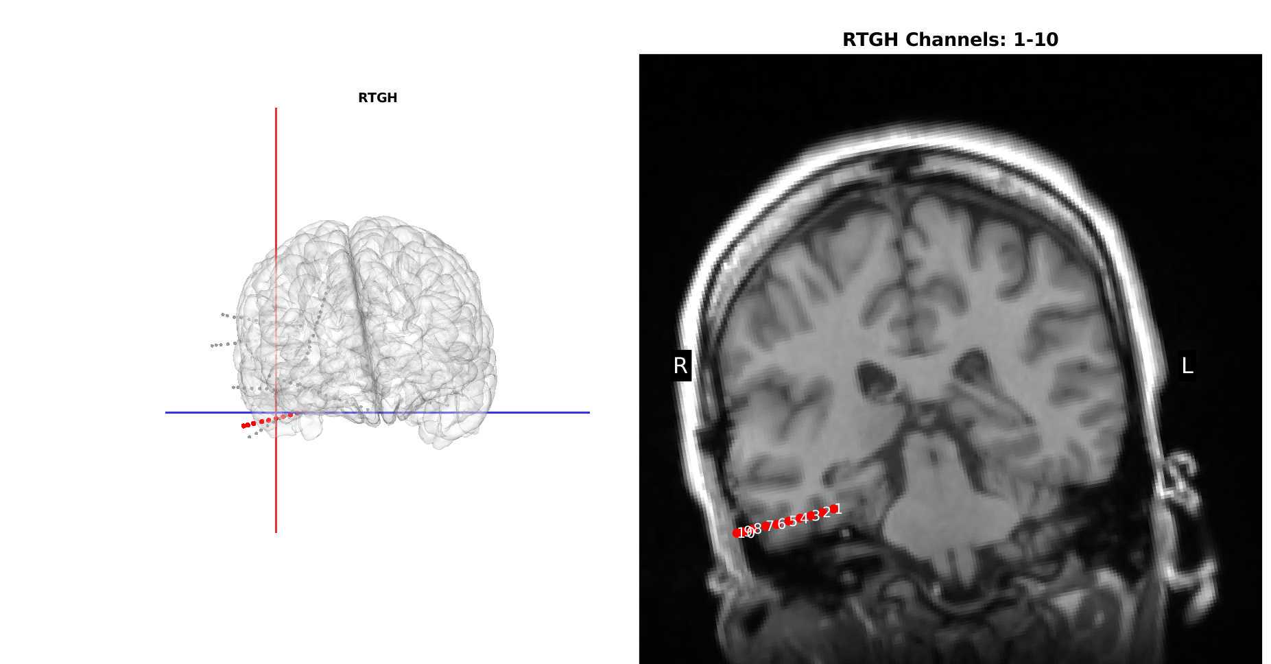
Create Images Per-Contact with MRIs and 3D Brains from all three views by clicking "Run Section" in the fourth and final section. This last section creates images for each electrode location superimposed on the MRI. This step may take many minutes depending on the number of electrodes.

On Linux, you can open a terminal in the “Images” folder and run this command if you install ImageMagick:

convert $(ls -v *.png) Recon.pdf

You can also use any PDF creation tool

Multi-Modality Visualization Tool (MMVT) and Electrode Labeling Algorithm (ELA)

If you are trying to run this part of the protocol with grids and strips, you need to separate every column or row of the grid to make it look like a separate depth (GR_##, GRa_##, GRb_##, etc). This is similar to the grid breakup from Step 5.4.

Navigate to your “mmvt_root” folder in a terminal. Activate the environment for MMVT and change directories:

source mmvt_env/bin/activate                                                                          cd mmvt_code

From now on, make sure you are running every line of code from the “mmvt_code” folder.

First, we must parcellate the brain surfaces based on a given atlas. Run this command to start the parcellation:

python -m src.preproc.anatomy --remote_subject_dir "Path/To/id##_SurferOutput" -s id##

It should take a few minutes. You’ll get a parcellation of the subject’s brain along with other surface files in “/…/mmvt_root/mmvt_blend/{ id## }” that will let you run the next step.

Run this command to run the Electrode Localization Algorithm (ELA):

python -m src.preproc.electrodes --remote_ras_fol "Path/To/id##_RAS Folder” --find_hemis_manual 1 -s id## -b 0
```-b 0 finds electrode locations for referential electrodes, -b 1 makes electrode locations for bipolar electrodes. Run as needed. 

* Add --overwrite_ela 1 to overwrite files already there
* If it says: “bad subject”, it’s usually fine. This just means not 100% of the algorithm ran. It will show different error messages if something important for ELA went wrong.
* --find_hemis_manual 1 turns on the ability to find the hemispheres for each electrode manually, though this will usually only require more input if you have grids and strips. You will have to type “l” or “r” for each electrode when prompted to indicate which hemisphere of the brain the electrode is in.


The important outputs of the electrode localization step are .csv files that contain the names of the electrode contact points in the first column and the subsequent columns—save for the last two—contain the probabilities that the a parcellated area of grey matter contains electrode contact points. The files are in /mmvt_root/mmvt_blend/[ **id\#\#** ]/electrodes, and they are labeled:



     **id\#\#** _aparc.DKTatlas40_electrodes_cigar_3_l_4.csv



        Or:

     **id\#\#** _aparc.DKTatlas40_electrodes_cigar_3_l_4_bipolar.csv





Again, the "-a" flag will be important for specifying the atlas. Please keep the -a flag consistent between the parcellation and the ELA steps. See Appendix VII for more information.

<Note title="Note" type="warning" ><span>Verifying the ELA output:</span><span></span><span>Look at probabilities for electrodes and make sure it makes sense for where they should be</span><span>If it fails, run with ela_overwrite 1 or you must delete files in these three locations to start over:</span><span>/home/cashlab/mmvt_root/electrodes//{<b>id##</b> }</span><span>/home/cashlab/mmvt_root/mmvt_blend/{<b>id##</b> } + files at the bottom </span><span>/home/cashlab/mmvt_root/electrodes_rois/electrodes</span></Note>

iEEG BIDS formatting of channel labels and file formats

A final step for the RAS file is to prepare the RAS channel data following FAIR practices (https://www.nature.com/articles/sdata201618) and the standard iEEG BIDS format (https://www.nature.com/articles/s41597-019-0105-7). For the iEEG BIDS formatting, manual entry to the RAS file for the electrode types (sEEG, grid, strip, or ECoG), electrode manufacturer, per-contact surface area (exposure to the brain), electrode group (e.g., the prefix label in front of electrode number), and the brain hemisphere. These details are recommended standard practice for information per RAS file, and, in our case, we made a copy and named this file:

“(patient designation)_ElectrodeInfo_RAS.xlsx” ( [https://www.nature.com/articles/s41597-019-0105-7](https://www.nature.com/articles/s41597-019-0105-7)).

The spreadsheet file along with other files can then be saved into the iEEG BIDS format, which involves following the BIDS file structure. Additional code is included (https://github.com/Center-For-Neurotechnology/Reconstruction-coreg-pipeline/tree/main/Deidentification_BIDSiEEG ) that uses the bids-starter kit code (https://bids-standard.github.io/bids-starter-kit/) and tailors it for this current format.

The spreadsheet file along with other files can then be saved into the iEEG BIDS format, which involves following the BIDS file structure. Additional code is included (https://github.com/Center-For-Neurotechnology/Reconstruction-coreg-pipeline/tree/main/Deidentification_BIDSiEEG ) that uses the bids-starter kit code (https://bids-standard.github.io/bids-starter-kit/) and tailors it for this current format.

For the shared example data sets, we then saved all the files into the iEEG BIDS format, placing the FreeSurfer output, the volumes per brain label (see below), and the MMVT output (see below) within the ‘derivatives’ folder. See the example data to follow the same data structure.

•Each participant is listed as sub-XXXX

•There are:

•per-participant files (highlighted in green)

•per-task files (highlighted in blue)

•There is the preimplant scan and postimplant scan (anat) with required .jsonfiles and both need to be defaced to deidentify the scans

•The file structure and naming matters and needs to be validated using BIDS-Validator: https://bids-standard.github.io/bids-validator/

•Information required and recommend in these files are listed here:

•https://bids-specification.readthedocs.io/en/stable/04-modality-specific-files/04-intracranial-electroencephalography.html

•And a tutorial here:

•https://bids-standard.github.io/bids-starter-kit/tutorials/ieeg.html

Measurements of electrode location relative to brain features

Following electrode localization, there are a number of different measures which could be relevant to further study, including localization relative to grey and white matter, different brain regions using a volumetric approach, contact size, and contact spacing. The organization of the FreeSurfer folders and RAS coordinates allow us to perform automatic calculations of these metrics using the current code.

A second type of labelling, electrode volume labelling (EVL), involves mapping electrode locations relative to volumes (as opposed to surfaces like ELA). To do this, we have to export the FreeSurfer parcellations to volumes, which involves using 3DSlicer (https://www.slicer.org/). The steps involve importing files from the surfer folder and then saving the volumes per brain label:

Load the brain.mgz and aparc.DKTatlas+aseg.mgzfiles (or whatever atlas you prefer) from the SurferOutput folder.

View the 3D render of the parcellations.

Save the output volumes of the parcellations: save (export) to the selected folder.

The resultant saved volumes can be used for later processing and mapping of electrode labels.

The next step involves involves running already created MATLAB code that uses the FreeSurfer, RAS, and MMVT file output structure to perform different calculations regarding electrode location, label electrodes based on the DKT40 atlas (https://mindboggle.info/data.html) or other selected brain atlas maps and produce output that matches the iEEG BIDS formatting. The code itself (Measurements_and_Labelling_RAS.m) performs the calculations and is dependent on the FreeSurfer and MMVT file structures and folder organization but, once organized, can just be run after pointing the script toward the correct participant designation. The code produces a spreadsheet (below), which includes further different measures and brain localization information. The code currently works with MATLAB 2020b onward though several of the functions can be run with older versions of MATLAB.

To remove identifying features, in addition to de-identifying the DICOM headers or re-saving the data as NIFTI files and removing the identifying header information, with instructions and approaches to do so outlined by various other sites (https://www.fieldtriptoolbox.org/).

An additional step is to remove facial features in the MRI and CT images and save the images into a format that can be read by steps in the pipeline such as FreeSurfer. This step involves using the Fieldtrip software and the functions ft_read_mri, ft_defacevolume, and the ft_write_mri functions. The procedure involves setting the path to the downloaded Fieldtrip code (see instructions on the Fieldtrip website) followed by running the functions pointing to the files and directories where the preoperative and postoperative images were located. The ft_defacevolumefunction opens up a graphic user interface (GUI) window that allows you to change he rotation and shape of the yellow box by entering numbers into the lower right corner of the box. Once you are satisfied the box covers the facial features for the scan, close the window which will result in saved anonymized MRI which can be saved using the ft_write_mri function.