Data normalisation of RT-qPCR data for detection of SARS-CoV-2 in wastewater
Adrian Roberts, Zhou Fang, Claus-Dieter Mayer, Anastasia Frantsuzova, Graeme J Cameron, Livia C T Scorza
Wastewater-based epidemiology
Infectious diseases
Public health
Covid-19
SARS-CoV-2
RNA viruses
sewage surveillance
normalisation
Abstract
After obtaining the raw measurements as gene copies per litre using RT-qPCR, a normalisation process is required prior to reporting the data as RNA copies per person.
This is because the concentration of viral RNA in wastewater is affected by both the population of the catchment area at each waterworks, as well as the amount of flow into the works. For example, an area with heavy rainfall will have high volumes of fluid flow, which will dilute RNA values.
Therefore, parameters such as the flow volume of wastewater and population size are used to overcome this bias.
Unfortunately, the flow data are not always accessible for all sites. Three methods were developed by Biomathematics and Statistics Scotland (BioSS) to estimate the flow for the normalization process, depending on data availability:
-
Normalisation using ammonia concentration to estimate flow;
-
Normalisation using flow historical average (when data for method 1 are not available);
-
Normalisation using predicted ammonia to estimate flow (when data for methods 1 and 2 are not available).
For all methods, the normalised outputs were reported as a daily value of RNA copies per person.
These methods are described separately in this protocol.
For other methodologies involving SARS-CoV-2 quantification in wastewater, such as viral RNA isolation and RT-qPCR, please refer to:
dx.doi.org/10.17504/protocols.io.bzv5p686 (RNA extraction from wastewater for detection of SARS-CoV-2 )
dx.doi.org/10.17504/protocols.io.bzwap7ae (RT-qPCR for detection of SARS-CoV-2 in wastewater)
Steps
Decision tree
Normalisation requires population size and water flow at the collection site.
Depending on the level of information available for particular site and date (such as ammonia content in wastewater or historical flow) different processing paths are available, as described below in the step by step algorithm.
The decision process is also described in the following figure
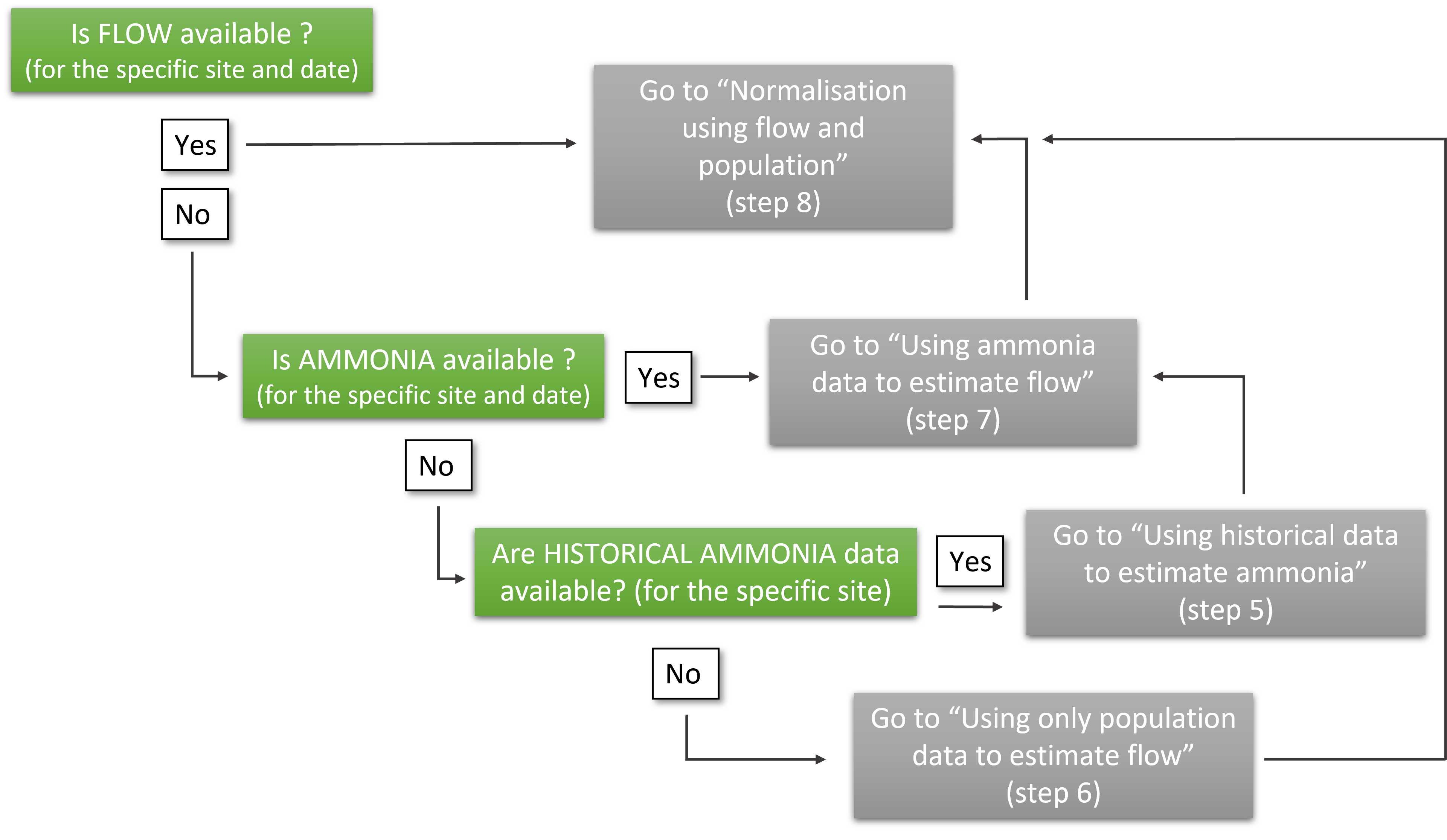
If flow data exist for a specific site and date (Flow[site, date]) GO TO normalisation step 8 ,
otherwise continue.
If flow data is not available, but measurements of ammonia concentration exist for a specific site and date (Am[site, date]) GO TO prediction step 7 ,
otherwise continue.
If there are no measurements for flow or ammonia concentration for a site on any dates GO TO step 5 , or, alternatively, go to step 6 if historical flow is available.
Using historical data to estimate ammonia
The missing amonia values can be infered from a generalized additive (GAM) spline model which fits sea``` minAm = min(Am) am_model = gam(log(Am + 1) ~ s(dates, k = 90) + sites) Am[site, date] = exp(predict(am_model, date, site)) - 1 Am = max(Am, minAm)
minAm = min(Am) am_model = gam(log(Am + 1) ~ s(dates, k = 90) + sites) Am[site, date] = exp(predict(am_model, date, site)) - 1 Am = max(Am, minAm)
 _Observations:_


 _- the smoothing parameter k=90 was chosen by preliminary analysis_


 _- the predicted value is prevented from being l_ ower than ever observed


GO TO to flow prediction step  **7**
Using only population data to estimate flow
If a site has no flow/ammonia data at all, use a national linear model based on population to predict flow
flow_model = lm(log10(Flow) ~ logPopulations)
pred = predict(flow_model, site_population)
Flow[site, date] = 10^pred
Observations:
- One has to take into account that by using flow historical average, the seasonal aspects are not considered, such as heavier rain fall in particular sites and seasons.
GO TO to normalisation step 8
Using ammonia data to estimate flow
When flow measurements are unavailable, but ammonia concentration in wastewater is available (directly or by estimation), a linear mixed statistical model can be used to estimate flow.
More specifically, a random coefficients model is used combining data from ammonia content and the population of each specific site. In this model the log of the flow is regressed on the log of the population and log of ammonia, which are used as fixed effects.
This model is used to calculate site specific coeficients, for those sites which have at least 25 dates with both ammonia and flow data availables. For the remaining sites the "fixed" effects are used.
flow_model = lmer(logflow ~ logpop + logammonia + (logammonia | site), REML=TRUE, data)
ammoniacoef[site] = coef(flow_model)[data_rich_sites]
ammoniacoef["Unknown"] = fixef(flow_model)
```The precomputed parameters are used to predict the flow (a table wth site specif coeficients is attached to this protocol).
param = ammoniacoef[site] || ammoniacoef["Unknown"]
Flow[site, date ] = 10^(param
 _Observations:_


 _- The coefficients parameters were update only every so often, with a degree of care like identifying outliers in the data._


[flow_mixed_model_coefficients_2021-08-10.csv](https://static.yanyin.tech/literature_test/protocol_io_true/protocols.io.b4eqqtdw/gr63bn7x72.csv)


GO TO to normalisation step  **8**
Normalisation using flow and population data
To produce a daily value of RNA copies per person, the raw RNA measurement is multiplied by the daily flow total, and divided by the population served at each site.
The flow for a specific site (waterworks location) is either measured directly or estimated using one of the methods from above.
normalized = gen_copies*Flow[site, date]/(site_population)/1e6 # unit [Mgc/p/d]
Code example
For illustration purposes we present the extract of the code for prediction of ammonia and flow which is used in the BioSS processing pipeline in R.
#normalisation - ammonia prediction
library(mgcv)

Rdate = as.Date(strptime(RNA$Date, "%m/%d/%Y"))
Rfdate = as.numeric(Rdate)[!is.na(RNA$Ammonia..mg.l.)]
Rfsite = factor(RNA$Site)[!is.na(RNA$Ammonia..mg.l.)]
RfAm = RNA$Ammonia..mg.l.[!is.na(RNA$Ammonia..mg.l.)]

flowobj = gam(log(RfAm + 1) ~ s(Rfdate, k = 90) + Rfsite) #k chosen by preliminary analysis

# flow ammonia model
wwdat$Flow-> FlowMean
Am = wwdat$Ammonia
Pop = rep((sitedata$PercentageNationalPop * sitedata$NationalPop)[isite], length(FlowMean))

# 0 = has flow, 1 = has only ammonia, 2 = has neither
dataType = is.na(FlowMean)*(1+ is.na(Am))
# do we have *any* flow/ammonia data for site?
if ((sum(!is.na(wwdat$Flow)) +sum(!is.na(wwdat$Am)) )>0){
	minAm = min(Am, na.rm=T)
	#fill in missing ammonias with ammonia from model
	if (sum(!is.na(Am)) > 0) Am[is.na(Am)] = exp(predict(flowobj, data.frame(Rfdate = as.numeric(as.Date(strptime(wwdat$Date,  "%m/%d/%Y"))), Rfsite = wwdat$Site))[is.na(Am)]) - 1
	Am = pmax(Am, minAm) #do not allow ammonia to go below minimum seen


	if (sitename %in% ammoniacoef$site){
		param = ammoniacoef[ammoniacoef$site == sitename,]
		# note adrian is based on log10 values, we reverse the reparameterisation
		pred = matrix(rep(10^(param$intercept+param$slope.lgpop*log10( param$Population )+param$slope.lgammonia*log10 (Am[is.na(wwdat$Flow)])), 3), ncol = 3)
	} else {
		# not in ammonia est, use unknown
		param = ammoniacoef[ammoniacoef$site == "Unknown",]
		pred = matrix(rep(10^(param$intercept+param$slope.lgpop*log10( Pop[1] )+param$slope.lgammonia*log10 (Am[is.na(wwdat$Flow)])), 3), ncol = 3)
	}
	FlowMean[is.na(wwdat$Flow)] = pred[,1]
	# if prediction fails use mean
	FlowMean[is.na(FlowMean)] = mean(FlowMean, na.rm = T)

} else {
	# if a site has no flow/am data at all, use a national linear model based on population
	logP = log10((sitedata$PercentageNationalPop * sitedata$NationalPop)[match(RNA$Site, sitedata$Simple)])

	pred = predict(lm(log10(RNA$Flow) ~logP), newdata = list(logP = log10(Pop)),interval = "prediction", level = WaterPredLev)
	FlowMean[is.na(FlowMean)] = 10^pred[,1]
}

var2 = wwdat$N1.Reported*FlowMean/(sitedata$PercentageNationalPop[isite]*sitedata$NationalPop[1]) /1e6 # calc Mgc/p/d

